Combining Stimuli in NRV

This example shows how logical and arithmetical operations on NRV’s stimulus object can facilitate the creation of complex stimulus.

• 
• 

1
500
3

import nrv
import numpy as np
import matplotlib.pyplot as plt

if __name__ == '__main__':
    model = 'Tigerholm'
    diam = 1
    y = 0
    z = 0
    print(diam)

    L = 10000

    t_sim = 50
    t_position=0.05
    t_start=20
    t_duration=1
    t_amplitude=1

    b_start = 3
    b_duration = t_sim
    block_amp = 20000
    block_freq = 10
    dt = 1/(20*block_freq)
    nseg_per_l = 50
    n_seg = np.int32(nseg_per_l*L/1000)
    print(n_seg)
    material = nrv.load_material('endoneurium_bhadra')

    y_elec = 500
    z_elec = 0
    x_elec = L/2

    axon1 = nrv.unmyelinated(y,z,diam,L,model=model,Nseg_per_sec=n_seg,dt=dt)


    E1 = nrv.point_source_electrode(x_elec,y_elec,z_elec)
    stim_1=nrv.stimulus()
    stim_1.sinus(b_start, b_duration, block_amp, block_freq ,dt=1/(block_freq*20))
    stim_extra = nrv.stimulation(material)
    stim_extra.add_electrode(E1,stim_1)
    axon1.attach_extracellular_stimulation(stim_extra)

    axon1.insert_I_Clamp(t_position, t_start, t_duration, t_amplitude)


    # simulate axon activity
    results = axon1.simulate(t_sim=t_sim)
    results.filter_freq('V_mem',block_freq)
    results.rasterize('V_mem_filtered')

    print(results.count_APs("V_mem_filtered"))

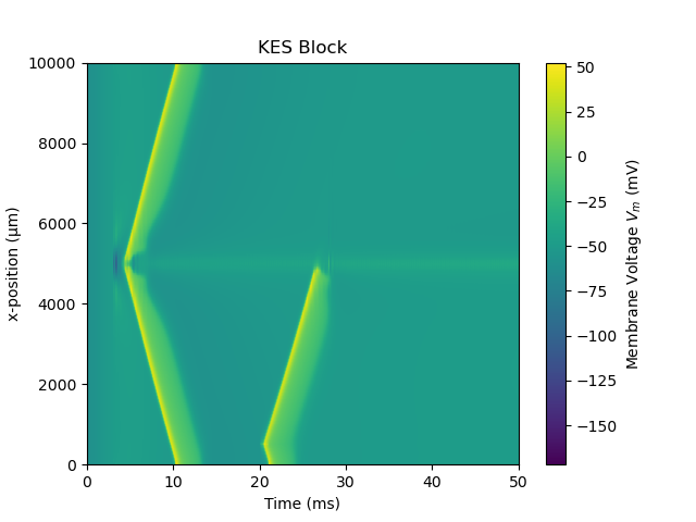
    fig, ax = plt.subplots(1)
    cbar = results.colormap_plot(ax, "V_mem_filtered")
    ax.set_xlabel('Time (ms)')
    ax.set_ylabel('x-position (µm)')
    ax.set_title('KES Block')
    cbar.set_label(r'Membrane Voltage $V_m$ (mV)')

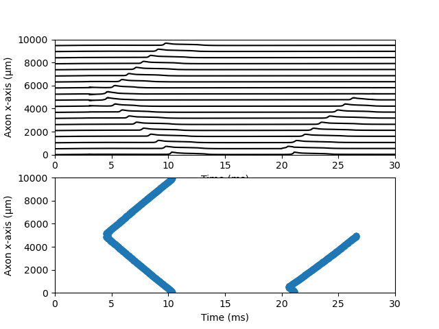
    fig, axs = plt.subplots(2)
    results.plot_x_t(axs[0],'V_mem_filtered')
    axs[0].set_ylabel("Axon x-axis (µm)")
    axs[0].set_xlabel("Time (ms)")
    axs[0].set_xlim(0,30)
    axs[0].set_ylim(0,np.max(results.x_rec))

    results.raster_plot(axs[1],'V_mem_filtered')
    axs[1].set_ylabel("Axon x-axis (µm)")
    axs[1].set_xlabel("Time (ms)")
    axs[1].set_xlim(0,30)
    axs[1].set_ylim(0,np.max(results.x_rec))

    plt.show()