Note
Go to the end to download the full example code.
Tutorial 4 - Stimulating Nerves with NRV
In this tutorial, we will create a nerve with two fascicles, populate it with axons, and stimulate it using both intra- and extra-fascicular electrodes.
As before, we start by importing the NRV package, along with numpy and matplotlib:
Note
As a best practice—especially when using multiprocessing—always place code execution inside a Python main guard:
if __name__ == "__main__":
    # your code here
This ensures compatibility across platforms and prevents unexpected behavior when spawning subprocesses. If you are running this tutorial as a .py file, remember to uncomment this line and indent all subsequent code accordingly.
import numpy as np
import matplotlib.pyplot as plt
import nrv

# if __name__ == "__main__":
Nerve creation
First, we need to create our nerve object using the NRV’s `nerve`-class. This object contains the geometrical properties of the nerve. NRV currently only supports cylindrical shapes for nerve, thus a diameter (`nerve_d`) and a length (`nerve_l`) must be specified at the nerve creation. The `Outer_D` parameter can also be specified. It refers to the saline solution bath diameter in which the nerve is plunged into.
Then, we will add two fascicles to the nerve. Fascicles in NRV combine a shape (CShape) and an axon population (axon_population). In addition, the `ID` parameter of the `fascicle` object tags each fascicle of the model, which will facilitate the post-simulation analysis.
Build fascicles’ geometry
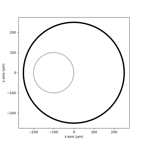
Fascicles can be defined with NRV’s `fascicle` class. Fascicles are incorporated one by one into the `nerve` object using the `add_fascicle` method. We can now plot a 2-D section of the nerve with the `plot` method of the `nerve` object to visualize it.
Fascicle’s shape from diameter
The simplest method is to define a circular fascicle by its diameter and its (y, z) coordinates in space.
Note
In our case, the (0, 0) coordinate is aligned with the center of the nerve. Its final position in the nerve is reached with a translation when added to the nerve.
Tip
An elliptic fascicle can also be generated with the quick method by setting diameter as a tuple (corresponding to the smallest and largest diameters of the ellipse). In such a case, an eventual rotation can be added using the rot argument of nerve.add_fascicle
fasc1_d = 200       # in um
fasc1_y = -100      # in um
fasc1_z = 0         # in um


#create the fascicle objects
fascicle_1 = nrv.fascicle(diameter=fasc1_d,ID=1)
nerve.add_fascicle(fascicle=fascicle_1, y=fasc1_y, z=fasc1_z)

#plot
fig, ax = plt.subplots(1, 1, figsize=(6,6))
nerve.plot(ax)
ax.set_xlabel("z-axis (µm)")
ax.set_ylabel("y-axis (µm)")
Text(22.972222222222214, 0.5, 'y-axis (µm)')
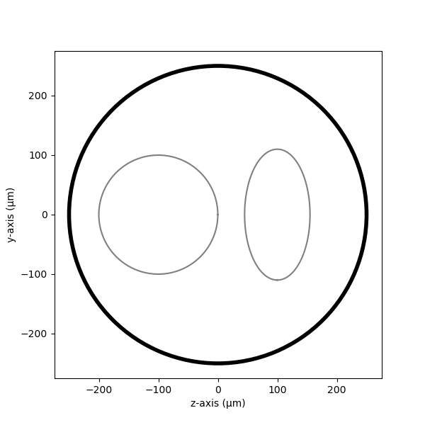
Fascicle’s shape from CShape
A second method to build a custom-shaped fascicle consists in using set_geometry().
In this example, we generate a second elliptic fascicle centered at $(y,z) = (100, 0)mu m$ with minor and major radii of $(110, 55)mu m$. The geometry is created using create_cshape().
Note
This time, as the fascicle is already positioned from its geometry, it is added to our nerve without any additional translation.
See also
Builtin geometry <../usersguide/geometry>. Example 18 <../examples/19_build_geometry>.
fasc2_d = (220,110)       # in um
fasc2_center = (100, 0)       # in um
geom2 = nrv.create_cshape(center=fasc2_center, diameter=fasc2_d, rot=90, degree=True)

fascicle_2 = nrv.fascicle(ID=2)
fascicle_2.set_geometry(geometry=geom2)

#Add the fascicles to the nerve
nerve.add_fascicle(fascicle=fascicle_2)

#plot
fig, ax = plt.subplots(1, 1, figsize=(6,6))
nerve.plot(ax)
ax.set_xlabel("z-axis (µm)")
ax.set_ylabel("y-axis (µm)")
Text(22.972222222222214, 0.5, 'y-axis (µm)')
Populate fascicles with axons
Now that our nerve geometry is created, it is time to populate them with axons. For each fascicle, axon populations of axons can be generated and handle using the axon_population-class attribute fascicle.axons. The creation of an usable population consist in two steps:
The population creation
The population placement
Population creation
The first step is to create the population. In this example, we will populate each fascicle with myelinated and unmyelinated axons, with a total of 100 axons in each fascicle.
To create a realistic axon diameter distribution, we use the NRV’s create_population()-method. The function can either take for arguments:
a list of diameter and axons type (0 for umyelinated, 1 for myelinated):
data
To generate the population custumisable data. Or, in our case:
the number of axon in the population
`n_ax`the proportion of unmyelinated fibers in the population
`percent_unmyel`the myelinated axon distribution
`M_stat`the unmyelinated axon distribution
`U_stat`
To generate population from statistical distributions Available myelinated and unmyelinated axon distributions are described in Axon population users’ guide.
This method build an pandas.DataFrame attribute stored in axon_population.axon_pop (or fascicle.axons.axon_pop in the fascicle) and containing two columns:
The axons diameters in $mu m$:
"diameters"The axons myelination status (0 for umyelinated, 1 for myelinated):
"types"
Population placement
# The second step is to place the generated axon population within the fascicle. This is done using the :meth:`~nrv.nmod.axon_population.place_population`-method. This method automatically assigns (y, z) coordinates to each axon, ensuring that all axons are positioned inside the fascicle geometry. The placement algorithm respects the ``delta`` parameter, which sets the minimum allowed distance (in $\mu m$) between axons and between axons and the fascicle border.
#
# .. note::
#     A distinction can be done between the distance between axons and the distance with the border by using respectively ``delta_in`` and ``delta_trace``.
#
# The resulting positions are stored in the ``"y"`` and ``"z"`` columns of the ``axon_pop`` DataFrame (i.e., ``fascicle.axons.axon_pop``).
# An additional boolean column ``"is_placed"`` is generated assessing if each axon could have been placed in the population. Thus, if the population is too large to fit within the fascicle given the specified ``delta`` (i.e. some lines of ``"is_placed"`` are ``False``), cooresponding axons will still exist in the population but will not be considered in the fascicle.
#
# .. seealso:
#     More detail on mask and subpopulation in :doc:`Axon population users' guide <../usersguide/populations>`.
#
# .. tip::
#     As Jupyter notebook offer a great viewer for ``pandas.DataFrame``, axon population can be well printed by adding the following line at the python cell: ```fascicle_1.axons.axon_pop```.


fascicle_1.axons.place_population(delta=5)

ax_pop = fascicle_1.axons # Storing the population for later
fascicle_1.axons.get_sub_population()
Placing... ━━━━━━━━━━━━━━━━━━━━━━━━━━━━━━━━━━━━━━━━ 100% 0:00:00
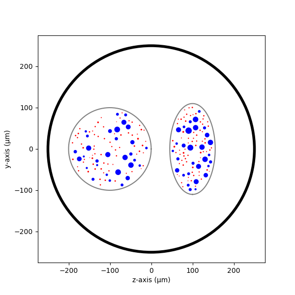
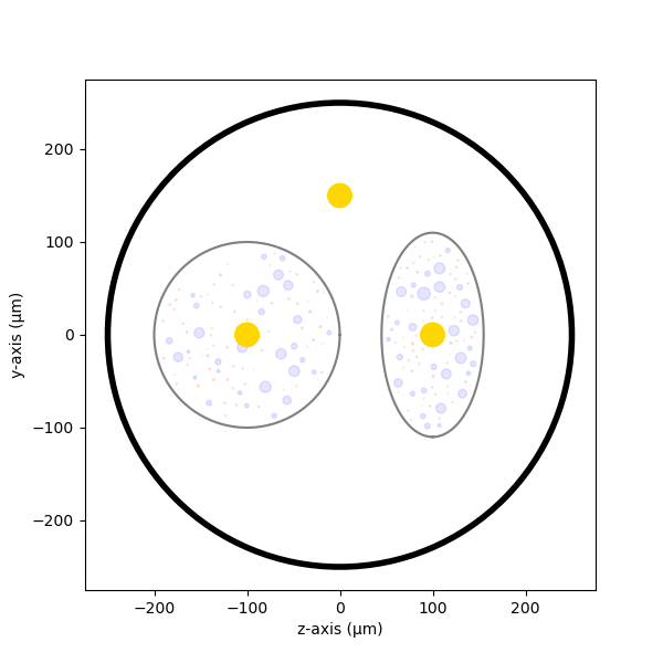
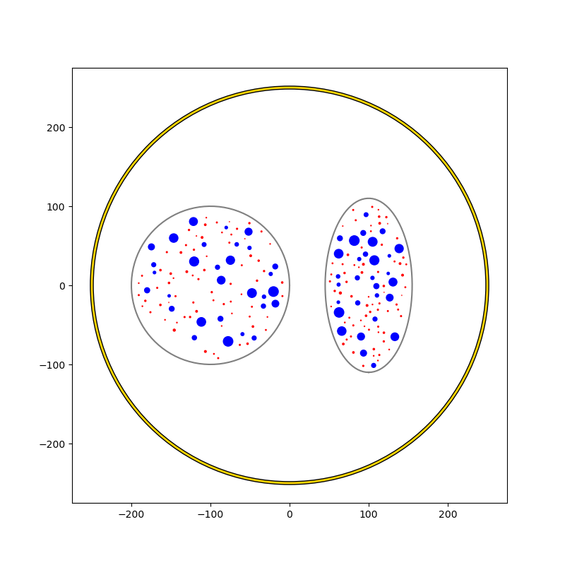
Let’s repeat this operation for the 2nd fascicle and plot the nerve again. This time, both creation and placement can be done in one line using the fascicle.fill-method.
Tip
This fascicle.fill-method is an alias for axon_population.fill_geometry, which calls create_population() and then place_population(). Its arguments are therefore the same as those of the two other methods.
Placing... ━━━━━━━━━━━━━━━━━━━━━━━━━━━━━━━━━━━━━━━━ 100% 0:00:00
We see that now our nerve is populated with fibers. Since the `fascicle_1```and ```fascicle_2`-objects are attached to the `nerve`-object, any modification to one of them will be propagated to the nerve.
fig, ax = plt.subplots(1, 1, figsize=(6,6))
nerve.plot(ax)
ax.set_xlabel("z-axis (µm)")
ax.set_ylabel("y-axis (µm)")
Text(22.972222222222214, 0.5, 'y-axis (µm)')
While we are here, we can also define stimulation parameters of the axons. For example, we can specify the computational model of the myelinated and unmyelinated fibers. You can refer to the previous tutorials for a thorough overview of the fiber’s simulation parameters available.
m_model = 'MRG'
um_model = 'Rattay_Aberham'
u_param = {"model": um_model}
m_param = {"model": m_model}

#For fascicle1
fascicle_1.set_axons_parameters(unmyelinated_only=True,**u_param)
fascicle_1.set_axons_parameters(myelinated_only=True,**m_param)

#For fascicle2
fascicle_2.set_axons_parameters(unmyelinated_only=True,**u_param)
fascicle_2.set_axons_parameters(myelinated_only=True,**m_param)
Extracellular stimulation context
Now we will define everything related to the extracellular stimulation. First, we need to create a `FEM_stimulation`-object. In this object, we can specify the conductivity of each material of the FEM stimulation. Available material conductivities are specified in Materials.
extra_stim = nrv.FEM_stimulation(endo_mat="endoneurium_ranck",      #endoneurium conductivity
                                peri_mat="perineurium",            #perineurium conductivity
                                epi_mat="epineurium",              #epineurium conductivity
                                ext_mat="saline")                  #saline solution conductivity
Adding intracellular electrodes
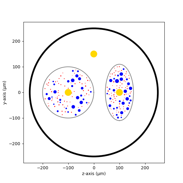
First, we will run some simulation with 3 intrafascicular LIFE-like electrodes, using the `LIFE_electrode` NRV’s object. In NRV, LIFEs are defined by a diameter (`life_d`), an active-site length (`life_length`) and a (x,y,z) spatial coordinates. A label and an ID can also be specified to facilitate post-simulation analysis. In this example we aligned the LIFEs x-position to the middle of the nerve, and set their (y,z) coordinates such that:
- `LIFE_0` is located inside the nerve but outside the fascicles
- `LIFE_1` is located inside `fascicle_1`
- `LIFE_2` is located inside `fascicle_2`
The electrodes are attached to the `extra_stim` `FEM_stimulation`-object with the `add_electrode`-method. The method also requires to link the electrode to a NRV `stimulus`-object. For that, we created a dummy stimulus ```dummy_stim```that we will change later.
life_d = 25                                 #LIFE diamter in um
life_length = 1000                          #LIFE active-site length in um
life_x_offset = (nerve_l-life_length)/2     #x position of the LIFE (centered)

life_y_c_0 = 0                              #LIFE_0 y-coordinate (in um)
life_z_c_0 = 150                            #LIFE_0 z-coordinate (in um)
life_y_c_1 = fasc1_y                        #LIFE_1 y-coordinate (in um)
life_z_c_1 = fasc1_z                        #LIFE_1 z-coordinate (in um)
life_y_c_2 = fasc2_center[0]                        #LIFE_2 y-coordinate (in um)
life_z_c_2 = fasc2_center[1]                        #LIFE_1 z-coordinate (in um)

elec_0 = nrv.LIFE_electrode("LIFE_0", life_d, life_length, life_x_offset, life_y_c_0, life_z_c_0, ID = 0) # LIFE in neither of the two fascicles
elec_1 = nrv.LIFE_electrode("LIFE_1", life_d, life_length, life_x_offset, life_y_c_1, life_z_c_1, ID = 1) # LIFE in the fascicle 1
elec_2 = nrv.LIFE_electrode("LIFE_2", life_d, life_length, life_x_offset, life_y_c_2, life_z_c_2, ID = 2) # LIFE in the fascicle 2

#Dummy stimulus
dummy_stim = nrv.stimulus()
dummy_stim.pulse(0, 0.1, 1)

#Attach electrodes to the extra_stim object
extra_stim.add_electrode(elec_0, dummy_stim)
extra_stim.add_electrode(elec_1, dummy_stim)
extra_stim.add_electrode(elec_2, dummy_stim)
Last, we attach `extra_stim`-object to the nerve with the `attach_extracellular_stimulation`-method:
nerve.attach_extracellular_stimulation(extra_stim)
Let’s see how our nerve with electrodes now looks like:
fig, ax = plt.subplots(1, 1, figsize=(6,6))
nerve.plot(ax)
ax.set_xlabel("z-axis (µm)")
ax.set_ylabel("y-axis (µm)")
Text(22.972222222222214, 0.5, 'y-axis (µm)')
The three LIFEs now are showing up, and we can make sure that their positions within the nerve are corrects. We also note that axon overlapping with the electrodes are removed.
Simulating the nerve
Now it’s time to run some simulations!
First, we set up a few flags:
- `nerve.save_results = False` disables the automatic saving of the simulation results in a folder
- `nerve.return_parameters_only = False` makes sure that all simulation results are returned to the `nerve_results```dictionnary.
- ```nerve.verbose = True` so it looks cool
Note
Saving simulation results in a folder and returning simulation parameters only can avoid excessive RAM memory usage for large nerve simulation. By default, nerve.save_results and `nerve.return_parameters_only` are set to False i.e. results are not saved in a folder and all simulation results are available in `nerve_results`.
Simulation duration is set with the `t_sim` parameter (in ms). We can also specify a `postproc_function` which will be applied to each axon’s simulation results. This is particularly useful to remove unused data and save up some memory. In this example we will use the `is_recruited` function..
Note
This cell takes several minutes to run.
nerve.save_results = False
nerve.return_parameters_only = False
nerve.verbose = True
nerve_results = nerve(t_sim=1,postproc_script = "is_recruited")         #Run the simulation
fascicle 1/2 -- 3 CPUs: 98 / 98 ━━━━━━━━━━━━━━━━━━━━━━━━━━━━━━━━━━━━━━━━ 100% 0:00:00 0:00:05
fascicle 2/2 -- 3 CPUs: 98 / 98 ━━━━━━━━━━━━━━━━━━━━━━━━━━━━━━━━━━━━━━━━ 100% 0:00:00 0:00:04
We can plot the nerve again and highlight axons that are recruited:
fig, ax = plt.subplots(1, 1, figsize=(6,6))
nerve_results.plot_recruited_fibers(ax)
ax.set_xlabel("z-axis (µm)")
ax.set_ylabel("y-axis (µm)")
Text(22.972222222222214, 0.5, 'y-axis (µm)')
No fiber activated are activated, of course the electrodes are stimulating with the `dummy_stim```stimulus! Let's change the stimulus of ```LIFE_2` (in `fascicle_2`) with a 100µs-long 60µA monophasic cathodic pulse:
t_start = 0.1       #start of the pulse, in ms
t_pulse = 0.1       #duration of the pulse, in ms
amp_pulse = 60      #amplitude of the pulse, in uA

pulse_stim = nrv.stimulus()
pulse_stim.pulse(t_start, -amp_pulse, t_pulse)      #cathodic pulse

fig, ax = plt.subplots()                            #plot it
pulse_stim.plot(ax) #
ax.set_ylabel("Amplitude (µA)")
ax.set_xlabel("Time (ms)")
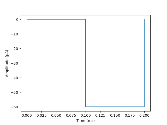
Text(0.5, 23.52222222222222, 'Time (ms)')
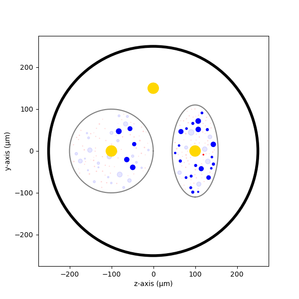
We can change the stimulus of `LIFE_2` by calling `change_stimulus_from_electrode` of the `nerve`-object with the `LIFE_2` ID and the new stimulus. We then re-run the simulation and plot the activated fibers.
nerve.change_stimulus_from_electrode(ID_elec=2,stimulus=pulse_stim)
nerve_results = nerve(t_sim=3,postproc_script = "is_recruited")

fig, ax = plt.subplots(1, 1, figsize=(6,6))
nerve_results.plot_recruited_fibers(ax)
ax.set_xlabel("z-axis (µm)")
ax.set_ylabel("y-axis (µm)")
fascicle 1/2 -- 3 CPUs: 98 / 98 ━━━━━━━━━━━━━━━━━━━━━━━━━━━━━━━━━━━━━━━━ 100% 0:00:00 0:00:08
fascicle 2/2 -- 3 CPUs: 98 / 98 ━━━━━━━━━━━━━━━━━━━━━━━━━━━━━━━━━━━━━━━━ 100% 0:00:00 0:00:07

Text(22.972222222222214, 0.5, 'y-axis (µm)')
Now we see some activation some fibers being recruited! All myelinated fibers in the `fascicle_2` are recruited, as few as a few unmyelinated ones. Some myelinated fibers are also recruited in `fascicle_1` but no unmyelinated ones. We can get the ratio of activated fiber in each fascicle using NRV’s built-in methods.
Note
Note that FEM is not recomputed between this simulation run and the previous. Indeed, as long as we don’t change any geometrical properties of the model, we only need to run the FEM solver once. This is automatically handled by the framework.
fasc_results = nerve_results.get_fascicle_results(ID = 1)                                #get results in fascicle 1
unmyel = fasc_results.get_recruited_axons('unmyelinated', normalize = True)              #get ratio of unmyelinated axon activated in fascicle 1
myel = fasc_results.get_recruited_axons('myelinated', normalize = True)                  #get ratio of myelinated axon activated in fascicle 1

print(f"Proportion of unmyelinated recruited in fascicle_1: {unmyel*100}%")
print(f"Proportion of myelinated recruited in fascicle_1: {myel*100}%")

fasc_results = nerve_results.get_fascicle_results(ID = 2)                                #get results in fascicle 2
unmyel = fasc_results.get_recruited_axons('unmyelinated', normalize = True)              #get ratio of unmyelinated axon activated in fascicle 2
myel = fasc_results.get_recruited_axons('myelinated', normalize = True)                  #get ratio of myelinated axon activated in fascicle 2

print(f"Proportion of unmyelinated recruited in fascicle_2: {unmyel*100}%")
print(f"Proportion of myelinated recruited in fascicle_2: {myel*100}%")
Proportion of unmyelinated recruited in fascicle_1: 7.246376811594203%
Proportion of myelinated recruited in fascicle_1: 17.24137931034483%
Proportion of unmyelinated recruited in fascicle_2: 33.33333333333333%
Proportion of myelinated recruited in fascicle_2: 79.3103448275862%
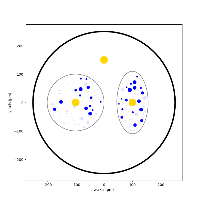
Let’s remove the stimulation in `LIFE_2` and apply it via `LIFE_0` instead:
nerve.change_stimulus_from_electrode(ID_elec=0,stimulus=pulse_stim)
nerve.change_stimulus_from_electrode(ID_elec=2,stimulus=dummy_stim)
nerve_results = nerve(t_sim=3,postproc_script = "is_recruited")
fascicle 1/2 -- 3 CPUs: 98 / 98 ━━━━━━━━━━━━━━━━━━━━━━━━━━━━━━━━━━━━━━━━ 100% 0:00:00 0:00:08
fascicle 2/2 -- 3 CPUs: 98 / 98 ━━━━━━━━━━━━━━━━━━━━━━━━━━━━━━━━━━━━━━━━ 100% 0:00:00 0:00:07
Let’s see how many fibers are activated now:
fasc_results = nerve_results.get_fascicle_results(ID = 1)                                #get results in fascicle 1
unmyel = fasc_results.get_recruited_axons('unmyelinated', normalize = True)              #get ratio of unmyelinated axon activated in fascicle 1
myel = fasc_results.get_recruited_axons('myelinated', normalize = True)                  #get ratio of myelinated axon activated in fascicle 1

print(f"Proportion of unmyelinated recruited in fascicle_1: {unmyel*100}%")
print(f"Proportion of myelinated recruited in fascicle_1: {myel*100}%")

fasc_results = nerve_results.get_fascicle_results(ID = 2)                                #get results in fascicle 2
unmyel = fasc_results.get_recruited_axons('unmyelinated', normalize = True)              #get ratio of unmyelinated axon activated in fascicle 2
myel = fasc_results.get_recruited_axons('myelinated', normalize = True)                  #get ratio of myelinated axon activated in fascicle 2

print(f"Proportion of unmyelinated recruited in fascicle_2: {unmyel*100}%")
print(f"Proportion of myelinated recruited in fascicle_2: {myel*100}%")

fig, ax = plt.subplots(figsize=(8, 8))
nerve_results.plot_recruited_fibers(ax)
ax.set_xlabel("z-axis (µm)")
ax.set_ylabel("y-axis (µm)")
Proportion of unmyelinated recruited in fascicle_1: 20.28985507246377%
Proportion of myelinated recruited in fascicle_1: 48.275862068965516%
Proportion of unmyelinated recruited in fascicle_2: 26.08695652173913%
Proportion of myelinated recruited in fascicle_2: 62.06896551724138%

Text(48.472222222222214, 0.5, 'y-axis (µm)')
We see that the recruitment profile in the fascicles is very different whether we stimulate with one or another electrode. We can analyze it by plotting recruitment curves.
Recruitment curves with LIFEs
To build the recruitment curve of our three electrodes, we are going to create a quick python function ```get_recruitment_electrode```that take as argument and electrode ID and a numpy array containing the pulse amplitude for the curve. The function return the ratio of myelinated and unmyelinated fibers recruited in each fascicle in python list.
def get_recruitment_electrode(elec_ID:int, amp_vec:np.array, nerve:nrv.nerve) -> list:

    nerve.verbose = False

    #create empty list to store results
    unmyel_fasc1,myel_fasc1,unmyel_fasc2,myel_fasc2 = ([] for i in range(4))

    #Deactivate unused electrodes
    elec_IDs = [0,1,2]
    unused_elec = [x for x in elec_IDs if elec_ID != x]
    for elec in unused_elec:
        nerve.change_stimulus_from_electrode(ID_elec=elec,stimulus=dummy_stim)

    #Loop throught amp_vec
    print(f"Stimulating nerve with LIFE_{elec_ID}")
    for idx,amp in enumerate(amp_vec):
        amp = np.round(amp,1)                                                       #get the amplitude
        print(f"Pulse amplitude set to {-amp}µA ({idx+1}/{len(amp_vec)})")
        pulse_stim = nrv.stimulus()                                                 #create a new empty stimulus
        pulse_stim.pulse(t_start, -amp, t_pulse)                                    #create a pulse with the new amplitude
        nerve.change_stimulus_from_electrode(ID_elec=elec_ID,stimulus=pulse_stim)    #attach stimulus to selected electrode
        nerve_results = nerve(t_sim=3,postproc_script = "is_recruited", pbar_off=True)             #run the simulation

        #add results to lists
        fasc_results = nerve_results.get_fascicle_results(ID = 1)
        unmyel_fasc1.append(fasc_results.get_recruited_axons('unmyelinated', normalize = True))
        myel_fasc1.append(fasc_results.get_recruited_axons('myelinated', normalize = True))
        fasc_results = nerve_results.get_fascicle_results(ID = 2)
        unmyel_fasc2.append(fasc_results.get_recruited_axons('unmyelinated', normalize = True))
        myel_fasc2.append(fasc_results.get_recruited_axons('myelinated', normalize = True))
    return(unmyel_fasc1,myel_fasc1,unmyel_fasc2,myel_fasc2)
We use this function to get the recruitment curve of each electrode with the cathodic pulse amplitude varying from 0µA to 150µA, in 20pts.
amp_min = 0             #start at 0µA
amp_max = 100           #ends at 100µA
n_amp = 20              #20pts
amp_vec = np.linspace(amp_min,amp_max,n_amp)
nrv.parameters.set_nmod_ncore(4)            #number of core allocated to fascicle simulations
unmyel_fasc1_LIFE0,myel_fasc1_LIFE0,unmyel_fasc2_LIFE0, myel_fasc2_LIFE0 = get_recruitment_electrode(0,amp_vec,nerve)
unmyel_fasc1_LIFE1,myel_fasc1_LIFE1,unmyel_fasc2_LIFE1, myel_fasc2_LIFE1 = get_recruitment_electrode(1,amp_vec,nerve)
unmyel_fasc1_LIFE2,myel_fasc1_LIFE2,unmyel_fasc2_LIFE2, myel_fasc2_LIFE2 = get_recruitment_electrode(2,amp_vec,nerve)

del nerve, extra_stim #to avoid meshing error, known bug
Stimulating nerve with LIFE_0
Pulse amplitude set to -0.0µA (1/20)


Pulse amplitude set to -5.3µA (2/20)


Pulse amplitude set to -10.5µA (3/20)


Pulse amplitude set to -15.8µA (4/20)


Pulse amplitude set to -21.1µA (5/20)


Pulse amplitude set to -26.3µA (6/20)


Pulse amplitude set to -31.6µA (7/20)


Pulse amplitude set to -36.8µA (8/20)


Pulse amplitude set to -42.1µA (9/20)


Pulse amplitude set to -47.4µA (10/20)


Pulse amplitude set to -52.6µA (11/20)


Pulse amplitude set to -57.9µA (12/20)


Pulse amplitude set to -63.2µA (13/20)


Pulse amplitude set to -68.4µA (14/20)


Pulse amplitude set to -73.7µA (15/20)


Pulse amplitude set to -78.9µA (16/20)


Pulse amplitude set to -84.2µA (17/20)


Pulse amplitude set to -89.5µA (18/20)


Pulse amplitude set to -94.7µA (19/20)


Pulse amplitude set to -100.0µA (20/20)


Stimulating nerve with LIFE_1
Pulse amplitude set to -0.0µA (1/20)


Pulse amplitude set to -5.3µA (2/20)


Pulse amplitude set to -10.5µA (3/20)


Pulse amplitude set to -15.8µA (4/20)


Pulse amplitude set to -21.1µA (5/20)


Pulse amplitude set to -26.3µA (6/20)


Pulse amplitude set to -31.6µA (7/20)


Pulse amplitude set to -36.8µA (8/20)


Pulse amplitude set to -42.1µA (9/20)


Pulse amplitude set to -47.4µA (10/20)


Pulse amplitude set to -52.6µA (11/20)


Pulse amplitude set to -57.9µA (12/20)


Pulse amplitude set to -63.2µA (13/20)


Pulse amplitude set to -68.4µA (14/20)


Pulse amplitude set to -73.7µA (15/20)


Pulse amplitude set to -78.9µA (16/20)


Pulse amplitude set to -84.2µA (17/20)


Pulse amplitude set to -89.5µA (18/20)


Pulse amplitude set to -94.7µA (19/20)


Pulse amplitude set to -100.0µA (20/20)


Stimulating nerve with LIFE_2
Pulse amplitude set to -0.0µA (1/20)


Pulse amplitude set to -5.3µA (2/20)


Pulse amplitude set to -10.5µA (3/20)


Pulse amplitude set to -15.8µA (4/20)


Pulse amplitude set to -21.1µA (5/20)


Pulse amplitude set to -26.3µA (6/20)


Pulse amplitude set to -31.6µA (7/20)


Pulse amplitude set to -36.8µA (8/20)


Pulse amplitude set to -42.1µA (9/20)


Pulse amplitude set to -47.4µA (10/20)


Pulse amplitude set to -52.6µA (11/20)


Pulse amplitude set to -57.9µA (12/20)


Pulse amplitude set to -63.2µA (13/20)


Pulse amplitude set to -68.4µA (14/20)


Pulse amplitude set to -73.7µA (15/20)


Pulse amplitude set to -78.9µA (16/20)


Pulse amplitude set to -84.2µA (17/20)


Pulse amplitude set to -89.5µA (18/20)


Pulse amplitude set to -94.7µA (19/20)


Pulse amplitude set to -100.0µA (20/20)
Now let’s look at the results for myelinated fibers:
c_LIFE_0 = "darkcyan"
c_LIFE_1 = "orangered"
c_LIFE_2 = "seagreen"

fig, (ax1, ax2) = plt.subplots(1, 2)

ax1.plot(amp_vec,myel_fasc1_LIFE0, '-o', lw=2, color= c_LIFE_0, label = 'LIFE_0')
ax1.plot(amp_vec,myel_fasc1_LIFE1, '-o', lw=2, color= c_LIFE_1, label = 'LIFE_1')
ax1.plot(amp_vec,myel_fasc1_LIFE2, '-o', lw=2, color= c_LIFE_2, label = 'LIFE_2')
ax1.set_title("Fascicle 1 - Myelinated")

ax2.plot(amp_vec,myel_fasc2_LIFE0, '-o', lw=2, color= c_LIFE_0, label = 'LIFE_0')
ax2.plot(amp_vec,myel_fasc2_LIFE1, '-o', lw=2, color= c_LIFE_1, label = 'LIFE_1')
ax2.plot(amp_vec,myel_fasc2_LIFE2, '-o', lw=2, color= c_LIFE_2, label = 'LIFE_2')
ax2.set_title("Fascicle 2 - Myelinated")

for ax in ax1, ax2:
    ax.set_xlabel('Amplitude (µA)')
    ax.set_ylabel('Recruitment')
    ax.legend()

fig.tight_layout()
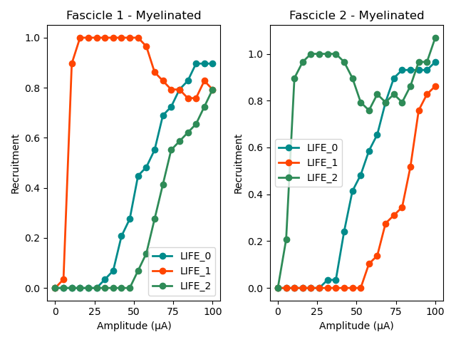
Myelinated fibers are progressively recruited when increasing the pulse amplitude. `LIFE_1` recruits the entire `fascicle_1` without recruiting any axon in `fascicle_2`. Oppositely, `LIFE_2` recruits the entire `fascicle_2` without recruiting any axon in `fascicle_1`. In other words, intrafascicular selective activation is possible with `LIFE_1```and ```LIFE_2`. `LIFE_0` however, located is neither of the two fascicles, can’t selectively activate one or the other fascicle.
Note
Proper curve analysis would require more simulation points. The presented result is for demonstration purposes only.
Let’s plot the unmyelinated fibers’ recruitment curves:
fig, (ax1, ax2) = plt.subplots(1, 2)
ax1.plot(amp_vec,unmyel_fasc1_LIFE0, '-o', lw=2, color= c_LIFE_0, label = 'LIFE_0')
ax1.plot(amp_vec,unmyel_fasc1_LIFE1, '-o', lw=2, color= c_LIFE_1, label = 'LIFE_1')
ax1.plot(amp_vec,unmyel_fasc1_LIFE2, '-o', lw=2, color= c_LIFE_2, label = 'LIFE_2')
ax1.set_title("Fascicle 1 - Unmyelinated")

ax2.plot(amp_vec,unmyel_fasc2_LIFE0, '-o', lw=2, color= c_LIFE_0, label = 'LIFE_0')
ax2.plot(amp_vec,unmyel_fasc2_LIFE1, '-o', lw=2, color= c_LIFE_1, label = 'LIFE_1')
ax2.plot(amp_vec,unmyel_fasc2_LIFE2, '-o', lw=2, color= c_LIFE_2, label = 'LIFE_2')
ax2.set_title("Fascicle 2 - Unmyelinated")

for ax in ax1, ax2:
    ax.set_xlabel('Amplitude (µA)')
    ax.set_ylabel('Recruitment')
    ax.legend()

fig.tight_layout()
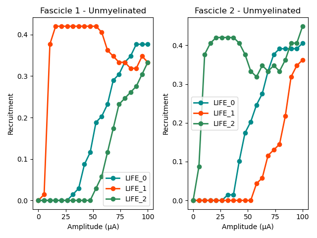
Activation of unmyelinated fibers requires much higher pulse amplitude. Electrodes located in the fascicle recruits at most about 10% of the unmyelinated fibers in `fascicle_1` and about 70% in `fascicle_2`. Electrode outside the fascicle or located in the other one fail at recruiting myelinated fibers.
Recruitment curves with a monopolar cuff-like electrode
Let’s create a second nerve with a cuff electrode now:
#creating the fascicles are populating them
fascicle_1_c = nrv.fascicle(diameter=fasc1_d,ID=1)
fascicle_2_c = nrv.fascicle(ID=2)
fascicle_2_c.set_geometry(geometry=geom2)

fascicle_1_c.fill(data=ax_pop[["types", "diameters"]], delta=5, fit_to_size=True)
fascicle_2_c.fill(data=ax_pop[["types", "diameters"]], delta=5, fit_to_size = True)

#set simulation parameters
fascicle_1_c.set_axons_parameters(unmyelinated_only=True,**u_param)
fascicle_1_c.set_axons_parameters(myelinated_only=True,**m_param)
fascicle_2_c.set_axons_parameters(unmyelinated_only=True,**u_param)
fascicle_2_c.set_axons_parameters(myelinated_only=True,**m_param)

#create the nerve and add fascicles
nerve_cuff = nrv.nerve(length=nerve_l, diameter=nerve_d, Outer_D=outer_d)
nerve_cuff.add_fascicle(fascicle=fascicle_1_c, y=fasc1_y, z=fasc1_z)
nerve_cuff.add_fascicle(fascicle=fascicle_2_c, y=fasc2_center[0], z=fasc2_center[1])

#set the simulation flags
nerve_cuff.save_results = False
nerve_cuff.return_parameters_only = False
nerve_cuff.verbose = True
Placing... ━━━━━━━━━━━━━━━━━━━━━━━━━━━━━━━━━━━━━━━━ 100% 0:00:00
Placing... ━━━━━━━━━━━━━━━━━━━━━━━━━━━━━━━━━━━━━━━━ 100% 0:00:00
We now create a FEM stimulation context, create a cuff electrode using the `CUFF_electrode`-class, combine everything and add it to the `nerve_cuff`-object:
extra_stim_cuff = nrv.FEM_stimulation(endo_mat="endoneurium_ranck",      #endoneurium conductivity
                                peri_mat="perineurium",            #perineurium conductivity
                                epi_mat="epineurium",              #epineurium conductivity
                                ext_mat="saline")                  #saline solution conductivity

contact_length=1000         # length (width) of the cuff contact, in um
contact_thickness=100       # thickness of the contact, in um
insulator_length=1500       # length (width) of the cuff insulator, on top of the contact
insulator_thickness=500     # thickness of the in insulator
x_center = nerve_l/2        # x-position of the cuff

cuff_1 = nrv.CUFF_electrode('CUFF', contact_length=contact_length,
    contact_thickness=contact_thickness, insulator_length=insulator_length,
    insulator_thickness=insulator_thickness, x_center=x_center)

extra_stim_cuff.add_electrode(cuff_1, dummy_stim)
nerve_cuff.attach_extracellular_stimulation(extra_stim_cuff)

fig, ax = plt.subplots(figsize=(8, 8))
nerve_cuff.plot(ax)
We can now simulate a recruitment curve with a cuff just like we did with the LIFE electrodes:
#create empty list to store results
unmyel_fasc1_cuff,myel_fasc1_cuff,unmyel_fasc2_cuff,myel_fasc2_cuff = ([] for i in range(4))

#Loop throught amp_vec
print("Stimulating nerve with CUFF")
for idx,amp in enumerate(amp_vec):
    amp = np.round(amp,1)                                                       #get the amplitude
    print(f"Pulse amplitude set to {-amp}µA ({idx+1}/{len(amp_vec)})")
    pulse_stim = nrv.stimulus()                                                 #create a new empty stimulus
    pulse_stim.pulse(t_start, -amp, t_pulse)                                    #create a pulse with the new amplitude
    nerve_cuff.change_stimulus_from_electrode(ID_elec=0,stimulus=pulse_stim)          #attach stimulus to selected electrode
    nerve_results = nerve_cuff(t_sim=3,postproc_script = "is_recruited", pbar_off=True)             #run the simulation

    #add results to lists
    fasc_results = nerve_results.get_fascicle_results(ID = 1)
    unmyel_fasc1_cuff.append(fasc_results.get_recruited_axons('unmyelinated', normalize = True))
    myel_fasc1_cuff.append(fasc_results.get_recruited_axons('myelinated', normalize = True))
    fasc_results = nerve_results.get_fascicle_results(ID = 2)
    unmyel_fasc2_cuff.append(fasc_results.get_recruited_axons('unmyelinated', normalize = True))
    myel_fasc2_cuff.append(fasc_results.get_recruited_axons('myelinated', normalize = True))
Stimulating nerve with CUFF
Pulse amplitude set to -0.0µA (1/20)


Pulse amplitude set to -5.3µA (2/20)


Pulse amplitude set to -10.5µA (3/20)


Pulse amplitude set to -15.8µA (4/20)


Pulse amplitude set to -21.1µA (5/20)


Pulse amplitude set to -26.3µA (6/20)


Pulse amplitude set to -31.6µA (7/20)


Pulse amplitude set to -36.8µA (8/20)


Pulse amplitude set to -42.1µA (9/20)


Pulse amplitude set to -47.4µA (10/20)


Pulse amplitude set to -52.6µA (11/20)


Pulse amplitude set to -57.9µA (12/20)


Pulse amplitude set to -63.2µA (13/20)


Pulse amplitude set to -68.4µA (14/20)


Pulse amplitude set to -73.7µA (15/20)


Pulse amplitude set to -78.9µA (16/20)


Pulse amplitude set to -84.2µA (17/20)


Pulse amplitude set to -89.5µA (18/20)


Pulse amplitude set to -94.7µA (19/20)


Pulse amplitude set to -100.0µA (20/20)
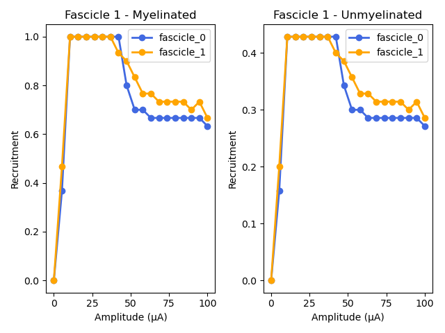
And plot the results:
c_fascicle_0 = "royalblue"
c_fascicle_1 = "orange"

fig, (ax1, ax2) = plt.subplots(1, 2)
ax1.plot(amp_vec,myel_fasc1_cuff, '-o', lw=2, color= c_fascicle_0, label = 'fascicle_0')
ax1.plot(amp_vec,myel_fasc2_cuff, '-o', lw=2, color= c_fascicle_1, label = 'fascicle_1')
ax1.set_title("Fascicle 1 - Myelinated")

ax2.plot(amp_vec,unmyel_fasc1_cuff, '-o', lw=2, color= c_fascicle_0, label = 'fascicle_0')
ax2.plot(amp_vec,unmyel_fasc2_cuff, '-o', lw=2, color= c_fascicle_1, label = 'fascicle_1')
ax2.set_title("Fascicle 1 - Unmyelinated")

for ax in ax1, ax2:
    ax.set_xlabel('Amplitude (µA)')
    ax.set_ylabel('Recruitment')
    ax.legend()

fig.tight_layout()
Total running time of the script: (20 minutes 8.088 seconds)