Scientific foundations

NRV is designed as an abstraction layer for the physical, mathematical, and computational techniques required for the realistic prediction and study of peripheral nerve’s electrical stimulation. The framework can be used with just a few lines of Python code on a wide range of computing platforms—from standard personal computers to high-performance supercomputers—without altering the simulation descriptions. It is also designed to interface seamlessly with optimization algorithms and experimental setups, facilitating the translation of novel stimulation protocols into experimental campaigns.

Framework overview

The NeuRon Virtualizer (NRV) is a fully open-source, multi-scale, and multi-domain Python-based framework developed for hybrid modeling of electrical stimulation in the Peripheral Nervous System (PNS). NRV shares the same core principle as other tools: a finite element method (FEM) model is solved under the quasi-static assumption to compute the extracellular potential generated by a stimulation source, which is then applied to a neural model to estimate the resulting neural activity.

However, NRV advances beyond other solutions by integrating all necessary steps for hybrid modeling directly within the framework—without relying on any commercially licensed software. Realistic electrode geometries and parameterized cylindrical nerves and fascicles are constructed and meshed using Gmsh [Geuzaine 2009], and FEM problems are solved using the open-source FEniCS software [Alnæs 2015]. An optional interface to COMSOL Multiphysics via COMSOL Server (commercial license required) is also implemented, offering users multiple options for 3D modeling.

Tools for generating realistic axon populations and placing them within the nerve structure are provided, along with widely used axon models from the literature. The extracellular potential computed via FEM is interpolated and used as input for 1D axon simulations. Intracellular stimulation (voltage or current clamp) can also be applied to one or more axons within an NRV model. Axon dynamics are simulated using NEURON, interfaced via its Python bridge. All inputs and outputs are stored in Python dictionary objects for easy context saving and data reuse. Post-processing tools are included to automatically detect action potentials, filter signals, and more. Extracellular recording devices can be added to simulate electrically evoked compound action potentials (eCAPs).

While optimization techniques have been successfully applied to improve electrode design [Kent 2013], stimulation waveforms [Yi 2020, Wongsarnpigoon 2010], and stimulation protocols [Cassar 2017], such approaches often require significant formalization and software development. NRV enhances these capabilities by providing a built-in formalism and a set of algorithms to describe and solve optimization problems for PNS simulations directly within the framework.

Regarding computational performance, NRV supports parallel processing. This accelerates axon simulation by enabling parallel execution of NEURON solvers. Parallelization is handled transparently and independently of the simulation logic—the user only needs to specify the number of available CPU cores, and NRV automatically manages task distribution and synchronization.

Calls to third-party software—Gmsh, FEniCS, COMSOL Server (for geometry definition, meshing, FEM solving, and field interpolation), NEURON (for neural simulations), or other tools used for post-processing—are fully encapsulated in NRV. No direct interaction with these libraries is needed, making the framework accessible to users with only basic Python skills, while remaining readable and flexible for advanced users.

NRV supports multi-scale simulations, from individual axon fibers to full-nerve models, all with minimal code. The framework is pip-installable and can be effortlessly deployed on computing clusters or supercomputers.

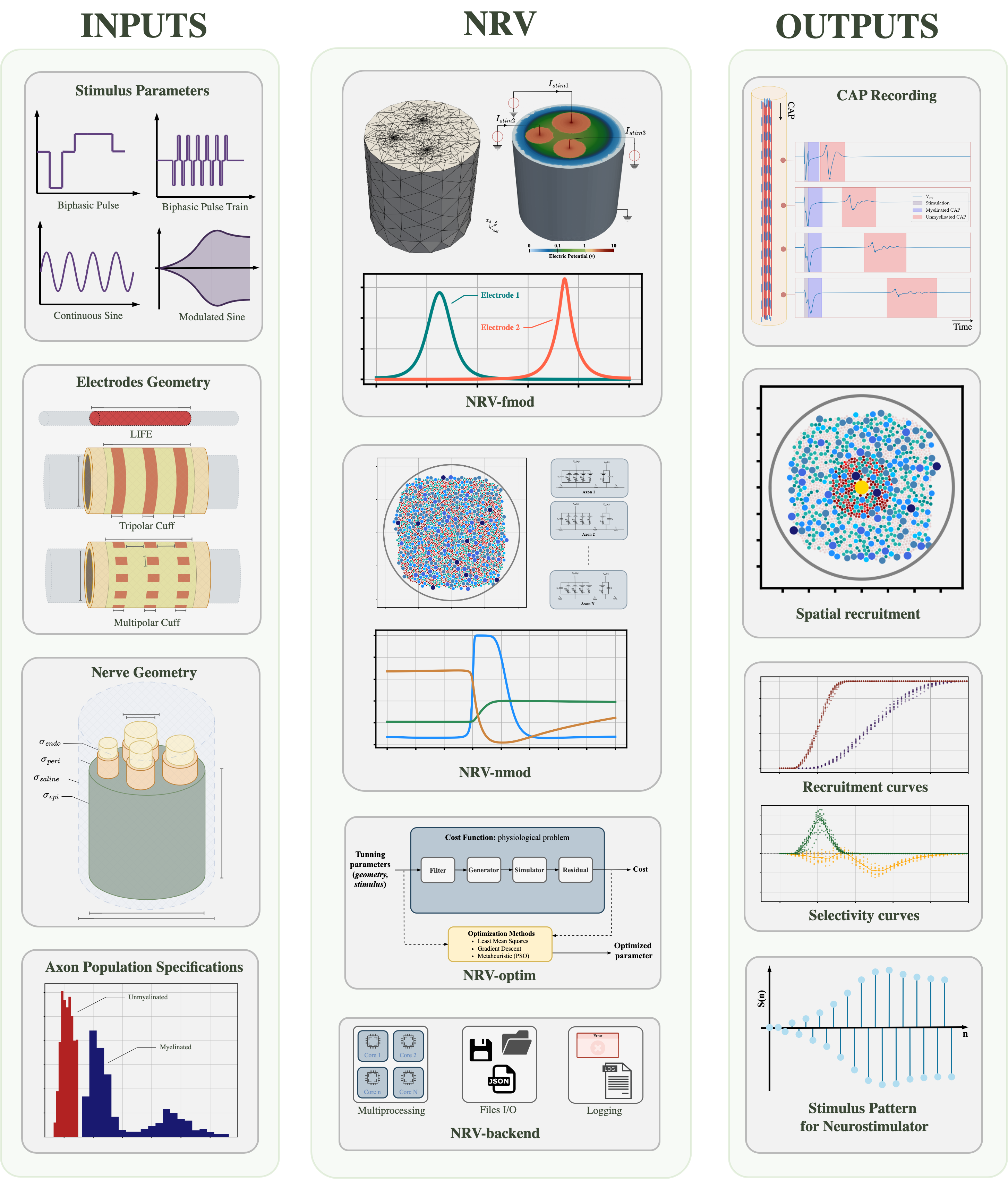
NRV’s internal architecture is illustrated in the figure above. It is divided into four main modules:

fmod – Manages extracellular models and field computations.
nmod – Handles axon membrane potential models and dynamics.
optim – Enables automatic optimization of stimulation contexts, including geometry and waveform parameters.
backend – Manages software engineering aspects such as hardware performance, parallel processing, and file I/O. This layer is essential to NRV’s operation but is abstracted away from the user and not described in detail.

fmod section: computation of 3D extracellular potentials

NRV provides tools, classes, and templates to define 3D models of nerves and electrodes. By default, all axons are aligned along the x-axis of the spatial frame. The figure below provides an overview of the simulated extracellular environment and a simplified UML class diagram showing accessible user-level components. This section details the physical implementation and computational methods.

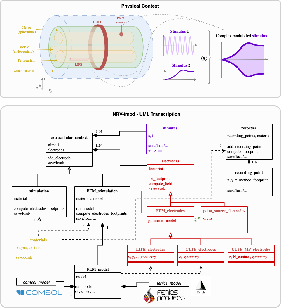
Computation of the extracellular potential for electrical stimulation is managed by the extracellular_context class. Its two main subclasses are:

analytical_stimulation – for analytical field solutions.
FEM_stimulation – for finite element simulations.

Both inherit from the common extracellular_context parent class, as shown in the figure above. NRV also supports analytical estimation of compound action potentials (CAPs) using recorder objects.

Electrical stimulation potential: computation mechanism

\[V_{ext}{\left( \mathbf{r}, t\right)} = \sum_{k\in E}{I_{stim_k}\left(t\right)V_{footprint_k}\left(\mathbf{r}\right)}\]

Where $E$ is the set of electrodes in the simulation, $I_{stim_k}$ is the stimulation current at electrode k, and $V_{footprint_k}$ is the precomputed potential footprint of electrode k for a unit current. The footprint represents the potential field generated in space by a unitary current injection and can be computed using either of the two methods described below.

The stimulation current $I_{stim_k}$ is defined via a stimulus object, which specifies time-current values applied to electrode k. Arithmetic operations between Stimulus objects are supported, allowing the construction of fully customized waveforms for complex protocols.

Upon creating an extracellular_context object, the user selects between the analytical or FEM method. This choice affects both computational demand and simulation realism. In both cases, users can add combinations of Electrode and Stimulus objects. Each Electrode has a unique ID, and multiple electrodes can be included.

With analytical_stimulation, only point-source electrodes are supported. This mode is intended for simulations without explicit geometry, where axons are embedded in a homogeneous medium.
With FEM_stimulation, models of cuff electrodes and longitudinal intrafascicular electrodes (LIFEs) are supported. These electrodes can be fully parameterized (e.g., number of contacts, size, spacing). Users can also define custom electrode geometries by subclassing the FEM_electrodes class. Electrode footprints are automatically computed when the extracellular_context is associated with axons.

Tissue electrical conductivities—either isotropic or anisotropic—are defined using the Material class. Predefined materials are available for epineurium, endoneurium, and perineurium based on commonly cited values [Ranck 1965], but custom conductivities can also be specified by the user.

Analytical evaluation of the extracellular potential

The analytical_stimulation-class solves the extracellular potential analytically using the PSA for the electrode, and the nerve is modeled as an infinite homogeneous medium [malmivuo1995]. This method is only suitable for geometry-less simulation: axons are considered as being surrounded by a unique homogeneous material. In this case, the footprint function is computed as:

\[V_{\text{footprint}} = \frac{1}{4\pi\sigma \vert\vert \mathbf{r} - \mathbf{r_e}\vert\vert}\]

where $\vert\vert \cdot \vert\vert$ denote the euclidean norm, $\mathbf{r_e}$ is the $\left( x_{e}, y_{e}, z_{e}\right)$ position of the PSA electrode and $\sigma`$ is the isotropic conductivity of the material. The conductivity of the endoneurium is generally considered as anisotropic [ranck1965specific] and is expressed as a diagonal matrix:

\[\begin{split}\boldsymbol{\sigma} = \begin{bmatrix} \sigma_{xx} & 0 & 0 \\ 0 & \sigma_{yy} & 0 \\ 0 & 0 & \sigma_{zz} \\ \end{bmatrix}\end{split}\]

The expression of the footprint function becomes [grill1999]:

\[V_{\text{footprint}} = \frac{1}{4\pi \sqrt{ \sigma_{yy}\sigma_{zz}(x - x_e)^2 + \sigma_{xx}\sigma_{zz}(y - y_e)^2+ \sigma_{xx}\sigma_{yy}(z - z_e)^2}}\]

The analytical approach provides a simple and quick estimation of the extracellular potential, allowing for fast computation on resource-constrained machines. However, it restricts the nerve geometry to an infinite homogeneous medium and omits the electrode shape and interface, limiting the viability of this approach for modeling complex experimental or therapeutic setups [mcintyre2001].

FEM computation of electrode footprints

The extracellular potential evaluation in a realistic nerve and electrode model using the FEM approach is handled by the FEM_stimulation-class. A nerve in NRV is modeled as a perfect cylinder and is defined by its diameter, its length, and the number of fascicles inside. The position and diameter of each fascicle on the NRV nerve can be explicitly specified. Fascicles of the NRV model are modeled as bulk volumes of endoneurium surrounded by a thin layer of perineurium tissue [pelot2018]. The remaining tissue of the nerve is modeled as a homogeneous epineurium. The nerve is plunged into a cylindrical material, which is by default modeled as a saline solution.

The NRV framework offers the possibility of using either COMSOL Multiphysics or FEniCS to solve the FEM problem. For the first one, mesh and FEM problems are defined in mph` files which can be parameterized in the FEM_stimulation-class to match the extracellular properties, and all physic equations are integrated into the Electric Currents` COMSOL library. When choosing FEniCS solver, NRV handles the mesh generation using Gmsh, the bridge with the solver, and the finite element problem with FEniCS algorithms. Physic equations solved are defined within the NRV framework. COMSOL Multiphysics is commonly used for the simulation of neural electrical stimulation investigation, but it requires a commercial license to perform computation, and all future developments are bound to the physics and features available in the software. We included the possibility of using it as a comparison to existing results but the use of FEniCS and Gmsh enables fully open-science and the possibility to enhance simulation possibilities and performances.

The electrode footprint $V_{footprint}$ is solved under quasi-static assumption in the simulation space $\Omega$. It is obtained from the Poisson equation, expressed as:

\[\mathbf{j}\left( \mathbf{r}\right) = \sigma\left( \mathbf{r}\right)\nabla V_{footprint}\left(\mathbf{r}\right), \forall \mathbf{r}\in \Omega\]

Where $\mathbf{j}$ is the current density and and $\sigma$ the electrical conductivity. Electrical ground is imposed on the outer surface of the saline solution using Dirichlet boundary condition. Neuman boundary conditions are used on the electrode active-sites. Dirichlet and Neuman boundary are defined as follow: $\mathbf{n}$

\[\begin{split}V_{footprint}\left(\mathbf{r}\right) = 0, \forall \mathbf{r} \in \partial \Omega_G \\ \sigma\left(\mathbf{r}\right) V_{footprint}\left(\mathbf{r}\right)\cdot \mathbf{n} = \mathbf{j_E}\left(\mathbf{r}\right), \forall \mathbf{r} \in \partial \Omega_E\end{split}\]

Where $\partial \Omega_G$ and $\partial \Omega_E$ are the electrical ground and the electrode active-site surface respectively, $\mathbf{n}$ the normal vector to $\partial \Omega_E$ and $\mathbf{j_E}$ the injected current density considered homogeneously distributed and expressed as:

\[\mathbf{j_E}\left(\mathbf{r}\right)\cdot\mathbf{n} = \frac{I_{stim}}{S_E}, \forall \mathbf{r} \in \partial\Omega_E\]

Where $I_{stim}$ is the stimulation current and $S_E$ is the electrode active site surface.

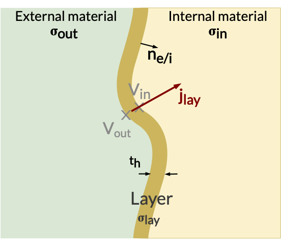
To reduce the number of elements in the mesh associated with smaller material dimensions, the fascicular perineurium volumes are defined using the thin-layer approximation (see Figure below) [givoli2004, pelot2018]. The current flow is assumed to be continuous through the layer, while a discontinuity is induced in the potentials:

\[\mathbf{j_{lay}} = \sigma _{in} \nabla V_{in} = \sigma _{out} \nabla V_{out} \mathbf{j_{lay}}\cdot \mathbf{n_{e/i}}= \frac{\sigma_{lay}}{t_h}(V_{in}-V_{out})\]

Simulation of eCAP recordings: computation mechanism

In NRV, eCAPs are computed analytically only, using a point- or line-source approximations (PSA or LSA) [parasuram2016] for the contribution of each axon in the simulation. Using the linear material impedance hypothesis, the total extracellular electrical potential can be considered as the sum of the contribution from the stimulating electrodes and the neural activity of the axon. Thus, the two contributions can be calculated separately. The geometry is only based on one material (by default endoneurium). This strategy ensures computational efficiency while still providing sufficiently quantitative results about axon synchronization and eCAP propagation for comparison with experimental observations.

The eCAP recording is performed automatically for the user when instantiating a recorder-object, which links one material with one or multiple recording-points-objects. recording-points-objects represents positions in space where the extracellular is recorded during the simulation. Using again space and time decoupling, the eCAP electrical potential at a position $\mathbf{r}$ at a time $t$ is computed as:

\[V_{eCAP}\left( \mathbf{r}, t\right) = \sum_{k\in\mathcal{A} } \sum_{i \in \mathcal{N}} I_{\text{mem }k,i}\left( t\right) V_{\text{footprint }k, i} \label{eq:eCAP}\]

where $\mathcal{A}$ is the set of axons in the simulation, $\mathcal{N}$ is the set of computational nodes in the axon implementation (see nmod section below), $I_{\text{mem }k,i}$ the membrane current computed in the nmod section(see below) and $V_{\text{footprint }k, i}$ is a scalar. From a numerical perspective, this equation is equivalent to a sum of dot products between two vectors: the membrane current computed in the nmod section of NRV (see below) and a recorder footprint. The footprint is computed only once for each axon in the nerve geometry before any simulation.

The footprint for one position $\mathbf{r_{k,i}} = \left( x_{k,i}, y_{k,i}, z_{k,i}\right)\in \mathbb{R}^3$ in space corresponding to the node $i$ of the axon $k$ for a recording-points-object at the position $r_{rec} =\left( x_{rec}, y_{rec}, z_{rec}\right) \in \mathbb{R}^3$ is computed either with PSA:

\[\begin{split}\begin{cases} V_{\text{footprint }k, i} = \dfrac{1}{4\pi \sqrt{\sigma_{yy}\sigma_{zz} x_d^2 + \sigma_{xx}\sigma_{zz} y_d^2+ \sigma_{xx}\sigma_{yy}z_d^2}}\\ x_d = (x_{k,i} - x_{rec})\\ y_d = (y_{k,i} - y_{rec})\\ z_d = (z_{k,i} - z_{rec}) \end{cases}\end{split}\]

for anisotropic or isotropic materials ($\sigma = \sigma_{xx} = \sigma_{yy} = \sigma_{zz}$), of with LSA for isotropic materials only [parasuram2016]

\[\begin{split}\begin{cases} V_{\text{footprint }k, i} = \dfrac{1}{4\pi \sigma \Delta l} \log{\dfrac{\sqrt{h_i^2 + r_i^2} - h_i}{\sqrt{l_i^2 + r_i^2} - l_i}} \\ \Delta l = \vert x_{k,i+1} + x_{k, l}\vert\\ r_i = \sqrt{(y_{k,i}-y_{rec})^2 + (z_{k,i}-z_{rec})^2}\\ h_i = \vert x_{k, i} - x_{rec}\vert \\ l_i = h_i + \Delta l \\ \end{cases}\end{split}\]

In both cases, the eCAP simulation is performed after the computation of neural activity, which is explained in the next section.

nmod section: generating and simulating axons

The description of a physiological context in NRV, as well as the computation of the axon membrane potential, are set up in a hierarchical manner described in the figure below. At the bottom of the hierarchy, axons are individual computational problems for which NRV computes an electrical response. As a conventional hypothesis, each axon is assumed independent from others, i.e., there is no ephaptic coupling between fiber, meaning that all axon computation can be done separately. From the computation aspect, this hypothesis transforms the neural computation to an embarrassingly parallel problem enabling massively parallel computations. In this section, details of models are given with a bottom-up approach: first axons models are described and explain up to nerves entities.

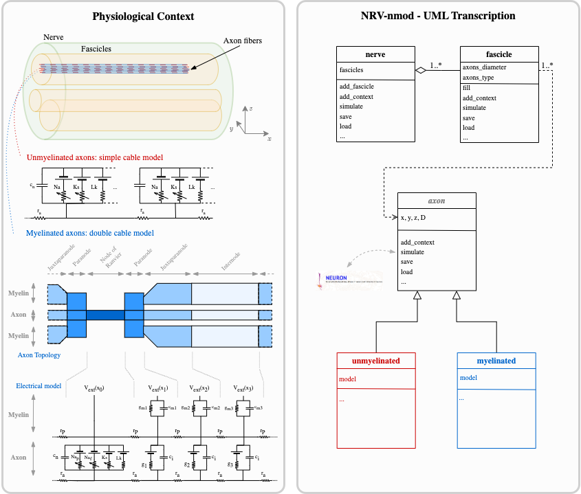
Axons models

Axonal fibers in NRV are defined with the axon-class. This class is an abstract Python class and cannot be called directly by the user. It however handles all generic definitions and the simulation mechanism. Axons are defined along the $x-axis$ of the nerve model. Axon (y,z) coordinates and length are specified at the creation of an axon-object. End-user accessible Myelinated-class and unmyelinated-class define myelinated and unmyelinated fiber objects respectively and inherit from the abstract axon-class.

Computational models can be specified for both the myelinated and unmyelinated fibers. Currently, NRV supports the MRG [mcintyre2002] and Gaines [gaines2018] models for myelinated fibers. It also supports the original Hodgkin-Huxley model [hodgkin1952quantitative], the Rattay-Aberham model [rattay1993modeling], the Sundt model [sundt2015spike], the Tigerholm model [tigerholm2014modeling], the Schild model [schild1994and] and its updated version [schild1997experimental] for unmyelinated fibers.

MRG and Gaines model’s electrical properties are available on ModelDB [hines2004modeldb] under accession numbers 3810 and 243841 respectively. Interpolation functions used in [gaines2018] to estimate the relationship between fiber diameter and node-of-Ranvier, paranode, juxtaparanodes, internode length, and axon diameter generate negative values when used with small fiber diameter. In NRV, morphological values from [mcintyre2002] and from [pelot2017modeling] are interpolated with polynomial functions. Parameters of the unmyelinated models are taken from [pelot2021excitation] and are available on ModelDB under accession number 266498.

The extracellular stimulations handled by the fmod-section of NRV are connected to the axon-object with the attach_extracellular_stimulation-method, linking the extracellular_context-object to the axon. Voltage and current patch-clamps can also be inserted into the axon model with the insert_V_Clamp-method and insert_I_Clamp-method. The simulate-method of the axon-class solves the axon model using the NEURON framework. NRV uses the NEURON-to-Python bridge [hines2009neuron] and is fully transparent to the user. The simulate-method returns a dictionary containing the fiber information and the simulation results.

Fascicle construction and simulation

The fascicle-class of NRV defines a population of fibers. The fascicle-object specifies the number of axons in the population, and the fiber type (unmyelinated or myelinated), the diameter, the computational model used, and the spatial location of each axonal fiber.

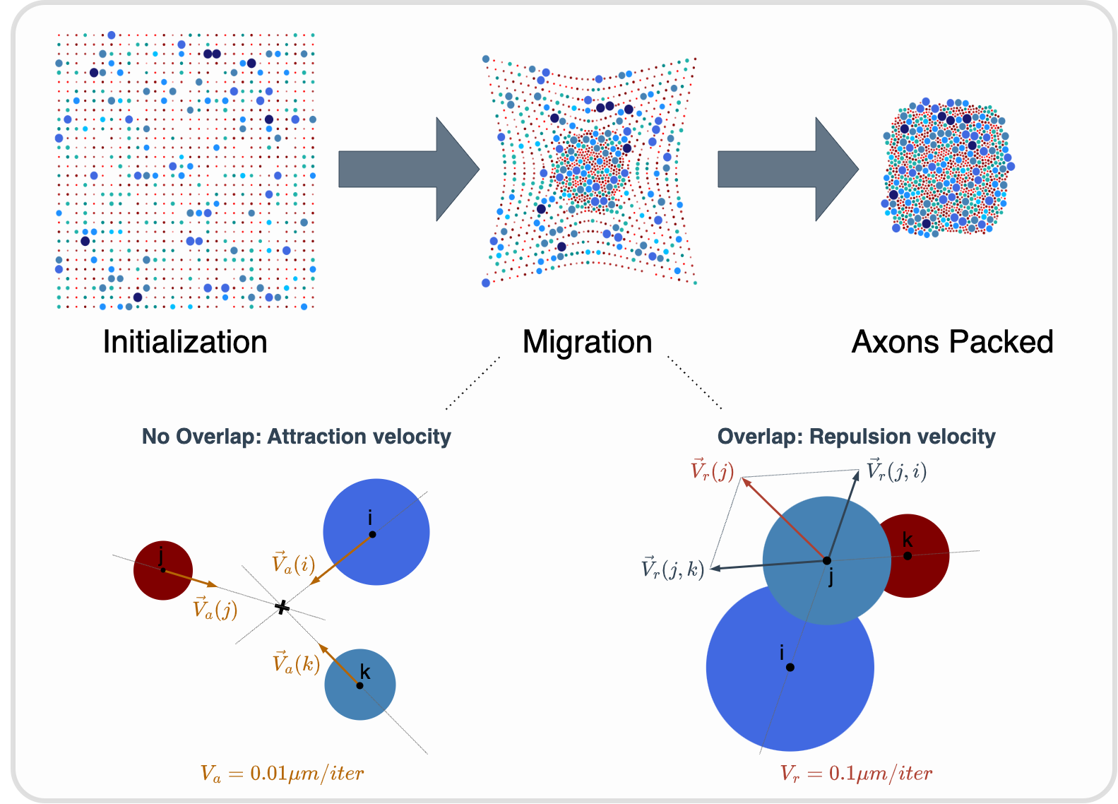
The axon population can be pre-defined and loaded into the fascicle-object. Third- party software such as AxonSeg (Zaimi et al. 2016) or AxonDeepSeg (Zaimi et al. 2018) can be used for generating axon populations from a histology section that are then loaded into the fascicle-object. Alternatively, the NRV framework provides tools to generate a realistic ex- novo population of axons. For example, the create_axon_population-function creates a population with a specified number of axons, a proportion of myelinated/unmyelinated fibers, and statistics for unmyelinated and myelinated fibers’ diameter repartition. Statistics taken from (Ochoa 1978; Jacobs and Love 1985; Schellens et al. 1993) have been interpolated and predefined as population-generating functions. User-defined statistics can also be specified. Alternatively, the fill_area_with_axons-function fills a user-specified area with axons according to the desired fiber volume fraction, fiber type, and diameter repartition statistics. To place cells inside the fascicle boundaries, an axon-packing algorithm is also included. The packing algorithm is inspired by (Mingasson et al. 2017). The generation of a realistic axon population and the packing principle are illustrated in the figure below.

The fascicle-class can perform logical and mathematical operations on the axon population. Operations include population rotation and translation and diameter or fiber-type filtering. Node-of-Ranvier of the myelinated fiber can be also aligned or randomly positioned in the fascicle. An extracellular_context-object is added to the fascicle-object using the attach_extracellular_stimulation-method. Intracellular stimulations can also be attached to the entire axon population or to a specified subset of fibers. The simulate- method creates an axon-object for each fiber of the fascicle, propagates the intracellular and extracellular stimulations and recorders, and simulates each of them. Parallelization of axons simulation is automatically handled by the framework and fully transparent to the user. The simulation output of each axon is saved inside a pre-defined folder.

Simulation top level: the nerve-object

The top-level nerve class is implemented to aggregate one or more fascicles and facilitate association with extracellular context. Fascicle-objects are attached to the nerve-object with the add_fascicle-method. The extracellular context is attached to the nerve-object and propagated to all fascicle-objects with the attach_extracellular_stimulation-method. The geometric parameters of the nerve-object and each fascicle-object are used to automatically generate the 3D model of the nerve. Calling the simulate-method of the nerve-object simulates each fascicle attached to the nerve and return either a Python dictionary containing all the results, or only the simulation parameters, with the results saved in a specified folder.

Optimizing a setup

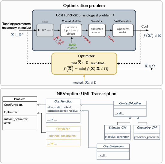
The figure above describes the generic formalism adopted in NRV for running optimization algorithms on PNS stimulations. The optimization problem, defined in a Problem-class, couples a Cost_Function-object, which evaluates the cost of the problem based on user-specified outcomes (e.g., stimulus energy, percentage of axon recruitment, etc.), to an optimization method or algorithm embedded in the Optimizer-object. The optimization space is defined by specifying in the problem definition the subset of available adjustable simulation parameters (e.g., stimulus shape, electrode size, etc.) and, optionally, their respective bounds.

NRV provides methods and objects to construct the Cost_Function-object according to the desired cost evaluation method and optimization space. Specifically, the Cost_Function-class is constructed around four main objects (see figure above):

A filter: which is an optional Python callable-object, for vector formatting or space restriction of the optimization space. In most cases, this function is set to identity and will be taken as such if not defined by the user.
A static context: it defines starting point of the simulation model to be optimized. It can be any of the nmod-objects (axon, fascicle, or nerve) to which all objects describing stimulation, recording and more generally the physical context are attached.
A context_modifier-object: it updates the static context according to the output of the optimization algorithm and the optimization space. The context_modifier-object is an abstract class, and two daughter classes for specific optimization problems are currently predefined: for stimulus waveform optimization or for geometry (mainly electrodes) optimization. However, there is no restriction to define any specific optimization scenario by inheriting from the parent context_modifier-class.
A cost_evaluation-object: uses the simulation results to evaluate a user-defined cost. Some examples of cost evaluation are included in the current version of the framework. Nonetheless, the cost_evaluation-class is a generic Python callable-class, so it can also be user-defined.

Optimization methods and algorithm implemented in NRV rely on third-party optimization libraries: SciPy optimize [2020SciPy-NMeth] for continuous problems, Pyswarms [pyswarmsJOSS2018] as Particle Swarms Optimization metaheuristic for high-dimensional or discontinuous problems.

References

[geuzaine2009] Geuzaine, C., & Remacle, J. F. (2009). Gmsh: A 3‐D finite element mesh generator with built‐in pre‐and post‐processing facilities. International journal for numerical methods in engineering, 79(11), 1309-1331.
[alnaes2015] Alnæs, M., Blechta, J., Hake, J., Johansson, A., Kehlet, B., Logg, A., … & Wells, G. N. (2015). The FEniCS project version 1.5. Archive of numerical software, 3(100).
[kent2013] Kent, A. R., & Grill, W. M. (2013). Model-based analysis and design of nerve cuff electrodes for restoring bladder function by selective stimulation of the pudendal nerve. Journal of neural engineering, 10(3), 036010.
[yi2020] Yi, G., & Grill, W. M. (2020). Kilohertz waveforms optimized to produce closed-state Na+ channel inactivation eliminate onset response in nerve conduction block. PLoS computational biology, 16(6), e1007766.
[wongsarnpigoon2010] Wongsarnpigoon, A., & Grill, W. M. (2010). Energy-efficient waveform shapes for neural stimulation revealed with a genetic algorithm. Journal of neural engineering, 7(4), 046009.
[cassar2017] Cassar, I. R., Titus, N. D., & Grill, W. M. (2017). An improved genetic algorithm for designing optimal temporal patterns of neural stimulation. Journal of Neural Engineering, 14(6), 066013.
[Ranck1965] Ranck Jr, J. B., & BeMent, S. L. (1965). The specific impedance of the dorsal columns of cat: an anisotropic medium. Experimental neurology, 11(4), 451-463.
[malmivuo1995] Malmivuo, J., & Plonsey, R. (1995). Bioelectromagnetism: principles and applications of bioelectric and biomagnetic fields. Oxford University Press, USA.
[grill1999] Grill, W. M. (1999). Modeling the effects of electric fields on nerve fibers: influence of tissue electrical properties. IEEE Transactions on Biomedical Engineering, 46(8), 918-928.
[mcintyre2001] McIntyre, C. C., & Grill, W. M. (2001). Finite element analysis of the current-density and electric field generated by metal microelectrodes. Annals of biomedical engineering, 29, 227-235.
[givoli2004] Givoli, D. (2004). Finite element modeling of thin layers. Computer Modeling In Engineering And Sciences, 5(6), 497-514.
[pelot2018] Pelot, N. A., Behrend, C. E., & Grill, W. M. (2018). On the parameters used in finite element modeling of compound peripheral nerves. Journal of neural engineering, 16(1), 016007.
[parasuram2016] Parasuram, H., Nair, B., D’Angelo, E., Hines, M., Naldi, G., & Diwakar, S. (2016). Computational modeling of single neuron extracellular electric potentials and network local field potentials using LFPsim. Frontiers in Computational Neuroscience, 10, 65.
[mcintyre2002] McIntyre, C. C., Richardson, A. G., & Grill, W. M. (2002). Modeling the excitability of mammalian nerve fibers: influence of afterpotentials on the recovery cycle. Journal of neurophysiology, 87(2), 995-1006.
[gaines2018] Gaines, J. L., Finn, K. E., Slopsema, J. P., Heyboer, L. A., & Polasek, K. H. (2018). A model of motor and sensory axon activation in the median nerve using surface electrical stimulation. Journal of computational neuroscience, 45, 29-43.