Stimuli
Electrical stimulation is fully described using electrodes that can deliver stimuli, which is the subject of the present chapter.
Electrical stimuli are electrical signals—mostly current values—applied extracellularly (and marginally intracellularly) to trigger cellular responses. In NRV, the stimulus has been designed to handle stimuli.
A stimulus is represented as an asynchronous signal: there is no need for a regular clock to describe the stimulus variations over time. Consequently, the stimulus is defined by two lists:
A first list, called
s, contains the signal values.A second list, called
t, contains the corresponding time stamps for these values.
The class constructor does not take positional arguments, but has one optional argument:
s_init: the initial value of the stimulus at timet = 0.
At instantiation, a stimulus is initialized only with its initial value at time t = 0, so the lists s and t both have a length of 1.
Here is a minimal example of stimulus instantiation:
It is possible to plot a stimulus instance using the plot() method, which takes Matplotlib axes as arguments. A more representative example of stimulus plotting is provided below in this chapter.
Stimuli Generators
The following table summarizes the available stimuli generators and their parameters:
Generator |
Parameter |
Description |
|---|---|---|
value (float) |
Value of the constant signal |
|
start (float) |
Starting time of the constant signal (default: 0) |
|
value (float) |
Value of the pulse |
|
start (float) |
Starting time of the pulse |
|
duration (float) |
Duration of the pulse (default: 0). If non-zero, a point is added at the end of the pulse with the previous value |
|
start (float) |
Starting time of the waveform, in ms |
|
s_cathod (float) |
Cathodic current in µA (always positive; absolute value) |
|
t_stim (float) |
Stimulation time, in ms |
|
s_anod (float) |
Anodic current in µA |
|
t_inter (float) |
Inter-pulse interval, in ms |
|
anod_first (bool) |
If true, anodic stimulation first; else cathodic first (default: False) |
|
start (float) |
Starting time, in ms |
|
duration (float) |
Duration, in ms |
|
amplitude (float) |
Amplitude in µA |
|
freq (float) |
Frequency in kHz |
|
offset (float) |
Offset current in µA (default: 0) |
|
phase (float) |
Initial phase in radians (default: 0) |
|
dt (float) |
Sampling step (0 = auto set for 100 samples per period) |
|
start (float) |
Starting time, in ms |
|
t_pulse (float) |
Pulse duration, in ms |
|
amplitude (float) |
Final amplitude in µA (absolute value) |
|
amp_list (list) |
Relative sine amplitudes (0 to 1) |
|
phase_list (list) |
Sine pulse phases |
|
dt (float) |
Sampling step (0 = auto set for 100 samples per period) |
|
start (float) |
Starting time, in ms |
|
duration (float) |
Duration, in ms |
|
amplitude (float) |
Amplitude in µA |
|
freq (float) |
Frequency in kHz |
|
offset (float) |
Offset current in µA (default: 0) |
|
anod_first (bool) |
If true, anodic stimulation first; else cathodic first (default: False) |
|
slope (float) |
Slope in µA·ms⁻¹ |
|
start (float) |
Starting time, in ms |
|
duration (float) |
Duration, in ms |
|
dt (float) |
Sampling step |
|
bounds (tuple) |
Boundary values of the ramp signal |
|
printslope (bool) |
If True, prints slope value (optional) |
|
ampstart (float) |
Initial amplitude, in µA |
|
ampmax (float) |
Maximum amplitude, in µA |
|
tstart (float) |
Starting time, in ms |
|
tmax (float) |
Ending time, in ms |
|
duration (float) |
Duration, in ms |
|
dt (float) |
Sampling step |
|
printslope (bool) |
If True, prints slope value (optional) |
As an example, let’s create a biphasic signal with a cathodic phase duration of \(50 \, \mu s\), a cathodic amplitude of \(1 \, \mu A\), a deadtime of \(40 \, \mu s\) between the cathodic and anodic phases, and a ratio of 5 between cathodic and anodic amplitudes. Additionally, we create a sinusoidal signal at \(1\, \mathrm{kHz}\) with an amplitude of 0.5.
import matplotlib.pyplot as plt

t_start = 1
V_cat = 1
t_cat = 60e-3   # recall, NRV's units are in ms
t_dead = 40e-3
ca_ratio = 5

biphasic_stim = nrv.stimulus()
biphasic_stim.biphasic_pulse(t_start, V_cat,t_cat, V_cat/ca_ratio, t_dead)

f_stim = 1      # recall, NRV's units are in ms
duration = 10
amp = 0.5

sinus_stim = nrv.stimulus()
sinus_stim.sinus(t_start, duration, amp, f_stim)


#print(dir(biphasic_stim))
fig, axs = plt.subplots(1, 2, layout='constrained', figsize=(10, 4))
biphasic_stim.plot(axs[0])
axs[0].set_title('Biphasic stimulus')
sinus_stim.plot(axs[1])
axs[1].set_title('Biphasic stimulus')
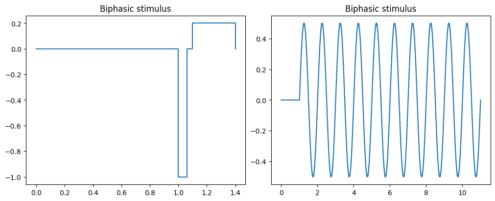
Note that the last value (here always 0) is not further plotted on the picture, however, the value is present in the table and in simulations, the last value of the stimuli is effectively applied to the electrode up until the end of simulation.
Mathematical operations with stimuli
The asynchronous description of stimuli is convenient for pulsed signals, such as those used with electrodes, and is also useful for handling simulations: ‘simulate’ methods are paused and stimulation is updated based on the time stamps of the involved stimuli.
However, this approach can also restrict operations with stimuli. To mitigate such restrictions, basic mathematical operations between stimulus objects have been implemented:
The operators
+,-, and*are implemented for use with numerical values or between two stimulus objects. Users do not need to worry about time stamp combinations. Note that division is not implemented, as it is ambiguous and may lead to divisions by zero. For division by a scalar, it is recommended to multiply by the inverse of that scalar.Absolute value (
abs) and negation of a stimulus are implemented.A length method (
len) is implemented.Equality and inequality comparison operators (
==,!=) are implemented. If stimuli are equal but not of the same length (i.e., successive equal values with multiple time stamps), the result is still straightforward. However, compared stimuli are not altered (redundancy of values is not removed). The operators<and>are not implemented as they are ambiguous.
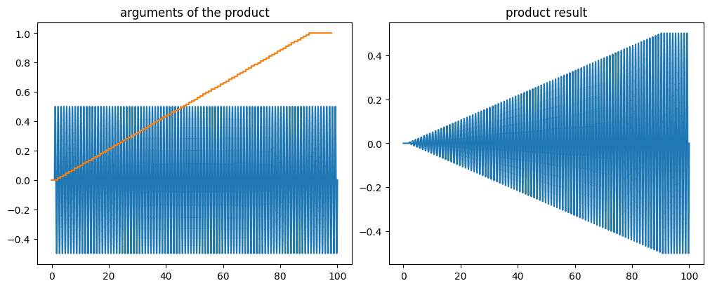
Below is an example of constant sinusoidal stimulation modulated by a ramp signal, demonstrating the use of these operations:
stim1, stim2 = nrv.stimulus(),nrv.stimulus()

f_stim = 1
t_start = 1
duration = 99
amp = 0.5

t_ramp_stop = 90
amp_start = 0
amp_max = 1

stim1.sinus(t_start, duration, amp, f_stim)
stim2.ramp_lim(t_start, t_ramp_stop, amp_start, amp_max, duration, dt=1)

stim3 = stim1*stim2
fig, axs = plt.subplots(1, 2, layout='constrained', figsize=(10, 4))

stim1.plot(axs[0])
stim2.plot(axs[0])
axs[0].set_title('arguments of the product')
stim3.plot(axs[1])
axs[1].set_title('product result')
Low level access
To develop new methods or functions, the user also has access to the following:
The
append()method, which takes as argument a pair consisting of a value and a time stamp.The
concatenate()method, which takes as arguments a pair of lists (or iterable, including NumPy arrays), with an optional argumentt_shiftthat shifts all time stamps by an offset (default is zero). This is especially useful for creating repetitive patterns.
An example is available and demonstrates the various signal generation possibilities in NRV.