Note
Go to the end to download the full example code.
Tutorial 6 - Play with EIT using NRV
Here is a tutorial showing the basic usage of nrv.eit sub-package.
See also
Further details on eit formalism can be found in usersguide’s EIT section.
- The tutorial is divided in 2 sections:
Note
This tutorial is inspired by the proof of principle of the application of EIT to imaging peripheral nerve activity, as published by K. Aristovich et al. in 2018
import nrv
import nrv.eit as eit
import numpy as np
import matplotlib.pyplot as plt
import os


test_id = "6"
res_dir  = f"./{test_id}/"
if "tutorials" in os.listdir():
    res_dir = "./tutorials" + res_dir[1:]

np.random.seed(4444)
Simulate the Measure (forward problem)
The main objective of this part is to simulate, for a given neural activity, the impedance change measured by multipolar cuff electrodes.
Setting parameters
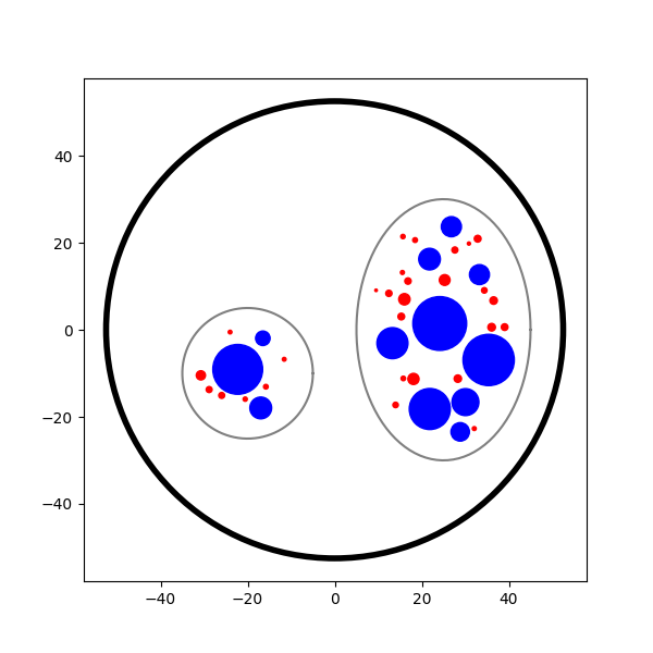
First, let’s define the nerve geometry for the simulation. As a case study, we can create a two-fascicle nerve as in a previous tutorial (see Tutorial 4).
Note
Here the generated nerve is only stored in a dict, but it could also be saved in a .json file and loaded afterwards.
outer_d = 5     # mm
nerve_d = 105  # um
nerve_l = 15010  # um
percent_unmyel = .7
unmyelinated_nseg = 3000
axons_data={
    "diameters":[10.001],
    "types":[1],
    "y":[0],
    "z":[0],
}

nerve_1 = nrv.nerve(length=nerve_l, diameter=nerve_d, Outer_D=outer_d, postproc_label="sample_keys", record_g_mem=True)

# Adding first fascicle
n_ax1=30
fasc1_d = (40, 60)   # um
fasc1_y = 25     # um
fasc1_z = 0     # um
fascicle_1 = nrv.fascicle(diameter=fasc1_d, ID=1, unmyelinated_nseg=unmyelinated_nseg)
fascicle_1.fill(n_ax=n_ax1, percent_unmyel=percent_unmyel, M_stat="Ochoa_M", U_stat="Ochoa_U", fit_to_size=False,delta=.5, delta_trace=3)
nerve_1.add_fascicle(fascicle=fascicle_1, y=fasc1_y, z=fasc1_z)

# Adding second fascicle
n_ax2=10
fasc2_d = 30   # um
fasc2_y = -20     # um
fasc2_z = -10     # um
fascicle_2 = nrv.fascicle(diameter=fasc2_d, ID=2, unmyelinated_nseg=unmyelinated_nseg)
fascicle_2.fill(n_ax=n_ax2, percent_unmyel=percent_unmyel, M_stat="Ochoa_M", U_stat="Ochoa_U", fit_to_size=False,delta=.5, delta_trace=3)
nerve_1.add_fascicle(fascicle=fascicle_2, y=fasc2_y, z=fasc2_z)

nerve_data = nerve_1.save(save=False)

fig, ax = plt.subplots(figsize=(6, 6))
nerve_1.plot(ax)

del nerve_1
Placing... ━━━━━━━━━━━━━━━━━━━━━━━━━━━━━━━━━━━━━━━━ 100% 0:00:00
Placing... ━━━━━━━━━━━━━━━━━━━━━━━━━━━━━━━━━━━━━━━━ 100% 0:00:00
Next, let’s define the simulation parameters for the EIT forward problem.
# This includes specifying the geometry, electrode configuration, stimulation protocol, and other relevant settings required to set up and run the finite element simulation of impedance measurements.

n_proc_global = 3


l_elec = 1000 # um
x_rec = 3000 # um
i_drive = 30 # uA
#dt_fem = 1 # ms
t_sim=10 # ms
t_iclamp = 0 # ms
n_fem_step = 10*n_proc_global

dt_fem = [
    (2, .75),
    (7,.4),
    (-1,.75),
        ]

n_elec = 16


sigma_method = "mean"
inj_protocol_type = "simple"
use_gnd_elec = True
parameters = {"x_rec":x_rec,
"dt_fem":dt_fem,
"inj_protocol_type":inj_protocol_type,
"n_proc_global":n_proc_global,
"l_elec":l_elec,
"i_drive":i_drive,
"sigma_method":sigma_method,
"use_gnd_elec":use_gnd_elec,
"n_elec":n_elec,
}
Run the simulation
EIT simulations can be done in three steps:
Nerve Simulation: Simulation of the neural context.
Mesh Generation: Creation of the problem geometry and physical domains.
EIT Simulation: Simulation of the electric field inside the nerve for a given injection protocol.
Note
These three steps, especially the latter, can be quite long. It can be interesting to adapt the number of process eiter
All these steps can be done from a single eit.EIT2DProblem-object.
Let’s start by instantiate the problem using the parameter set above.
Tip
You can find a list of tunable attribute in the API documentation (see nrv.eit.EIT2DProblem)
eit_instance = eit.EIT2DProblem(nerve_data, res_dname=res_dir, label=test_id, **parameters)
No such directory ./6/. Creating it to save the results
Nerve Simulation
As mention, the first step consist at simulated the electrical conductivity change of axons’ membrane induced by the activity. This can be done by calling nrv.eit.eit_forward.simulate_nerve()-method.
Tip
The arguments can be more simply understood as the combinaison of three arguments of the nrv.nmod.nerve-class: nrv.nrv.nmod.nerve.insert_I_Clamp(), nrv.nmod.nerve.set_axons_parameters() and nrv.nmod.nerve.simulate().
Basically, this method:
Adapt the nerve-object to match with the problem parameter.
Attach a current clamp to axons in the nerve.
Attach analytical recording points at the center of each electrode
Run the nerve simulation storing the axons’ membrane conductivity values for each temporal step of the FEM simulation.
If specified, save the simulation results in a .json file (in
nrv.eit.eit_forward.nerve_res_file).
Note
A customized on the flight post-processing is used to only store required values of membranes conductivity (see nrv.eit.utils.sample_nerve_results()).
fascicle 1/2 -- 3 CPUs: 30 / 30 ━━━━━━━━━━━━━━━━━━━━━━━━━━━ 100% 0:00:00 0:01:14
fascicle 2/2 -- 3 CPUs: 10 / 10 ━━━━━━━━━━━━━━━━━━━━━━━━━━━ 100% 0:00:00 0:00:39
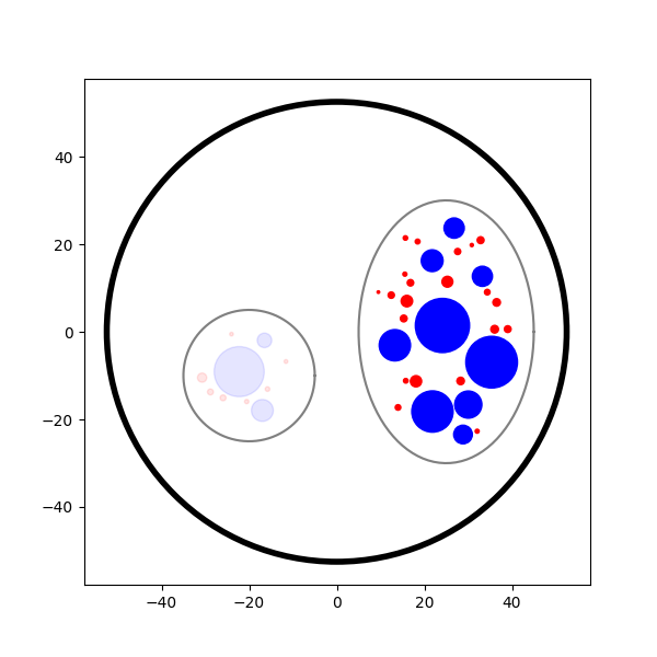
Let’s now plot the nerve highlighting the fibres activated during the simulation, as done in Tutorial 4.
fig, ax = plt.subplots(figsize=(6, 6))
nrn_res.plot_recruited_fibers(ax)
FEM Problem
Once the nerve simulation is complete, the goal of the following steps is to compute how changes in axonal membrane conductivity affect impedance measurements from extracellular electrodes. This is achieved by using FEM to calculate the electric field inside the nerve over time, for a given current injection between a pair of electrodes.
Although this process may seem complex, it has been fully integrated into the eit_forward class and can be performed in three lines:
nrv.eit.eit_forward._setup_problem(): Sets up the FEM problem using the geometrical and electrical properties stored in thenrv.nmod.results.nerve_resultsoutput from the nerve simulation.
Warning
This step may be merged with the next one in future versions of NRV.
nrv.eit.eit_forward.build_mesh(): Builds the mesh corresponding to the nerve geometry, including the multipolar cuff electrodes.nrv.eit.eit_forward.simulate_eit(): Runs the FEM simulation over all time, frequency, and drive pattern steps.
Note
Currently, the mesh is always saved in a .msh file (see nrv.eit.eit_forward.nerve_res_file) and reloaded at the beginning of each process during the simulation. This behaviour may change in future versions of NRV.
## Impedance simulation
eit_instance._setup_problem()
# Build mesh
eit_instance.build_mesh()

# Simulate nerve
fem_res = eit_instance.simulate_eit()
process 1 -- 3 : 112/112 ━━━━━━━━━━━━━━━━━━━━━━━━━━━━━━━━━━ 100% 0:00:00 0:00:38
process 2 -- 3 : 112/112 ━━━━━━━━━━━━━━━━━━━━━━━━━━━━━━━━━━ 100% 0:00:00 0:00:38
process 3 -- 3 : 112/112 ━━━━━━━━━━━━━━━━━━━━━━━━━━━━━━━━━━ 100% 0:00:00 0:00:38
The object returned by the EIT simulation is an instance of nrv.eit.results.eit_forward_results. The main purposes of this class are to:
Store the results of the simulations.
Facilitate access to specific results.
Provide post-processing and plotting tools to analyze the results.
Similar to other results classes in NRV, this class inherits from dict. However, to limit memory usage, only the following keys are stored:
“t”: Time vector of the FEM simulation results.
“f”: Frequency vector of simulation results.
“p”: Drive protocol used in the simulation.
“v_eit”: Voltage measurements magnitude from the EIT simulation.
“v_eit_phase”: Phase of the voltage measurements.
“t_rec”: Time vector of the nerve simulation results (for analytical recording).
“v_rec”: Voltage values recorded by the analytical recorders.
In this tutorial, we primarily use the results to feed the inverse problem and perform image reconstruction. Therefore, the various post-processing tools implemented in this class will not be detailed here.
See also
EIT users’ guide.
Examples.
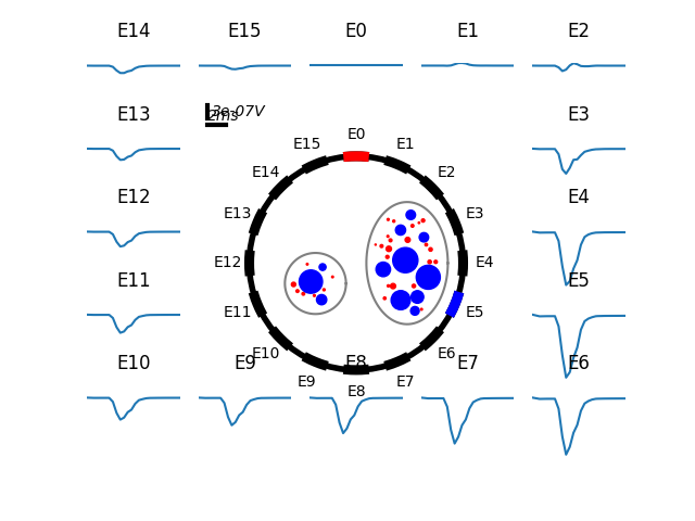
Let’s plot the impedance shift measured at each electrode over time for one drive pattern to better understand what have been simulated.
pat = fem_res["p"][0]
dv_pc = fem_res.dv_eit(i_p=0)

fig = plt.figure()
_, axs2 = eit.utils.gen_fig_elec(n_e=fem_res.n_e, fig=fig, )

eit.utils.add_nerve_plot(axs=axs2, data=nerve_data, drive_pair=pat)
eit.utils.plot_all_elec(axs=axs2, t=fem_res.t(), res_list=dv_pc,)
eit.utils.scale_axs(axs=axs2, e_gnd=[0], has_nerve=True)
[<Axes: title={'center': 'E0'}>, <Axes: title={'center': 'E1'}>, <Axes: title={'center': 'E2'}>, <Axes: title={'center': 'E3'}>, <Axes: title={'center': 'E4'}>, <Axes: title={'center': 'E5'}>, <Axes: title={'center': 'E6'}>, <Axes: title={'center': 'E7'}>, <Axes: title={'center': 'E8'}>, <Axes: title={'center': 'E9'}>, <Axes: title={'center': 'E10'}>, <Axes: title={'center': 'E11'}>, <Axes: title={'center': 'E12'}>, <Axes: title={'center': 'E13'}>, <Axes: title={'center': 'E14'}>, <Axes: title={'center': 'E15'}>, <Axes: >]
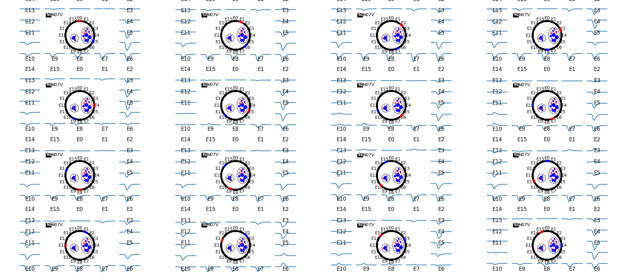
The previous plot can be extended to all injection patterns. However, for a 16-electrode protocol, the resulting image is not very readable.
if n_elec in [8, 16]:
    fig = plt.figure(figsize=(20, 9))
    subfigs = fig.subfigures(n_elec//4, 4)
    axs = np.array([])
    for i_p, pat in enumerate(fem_res["p"]):
        dv_pc = fem_res.dv_eit(i_p=i_p)
        _, axs2 = eit.utils.gen_fig_elec(n_e=fem_res.n_e, fig=subfigs[i_p//4, i_p%4], small_fig=True)
        eit.utils.add_nerve_plot(axs=axs2, data=nerve_data, drive_pair=pat)
        eit.utils.plot_all_elec(axs=axs2, t=fem_res.t(), res_list=dv_pc,)
        axs = np.concatenate([axs, axs2[1:-1]])
        eit.utils.scale_axs(axs=axs2, e_gnd=[0], has_nerve=True)
Tip
As mention above, only the voltage measured by the electrode is saved in eit_forward_results. To better understand the computed results, or to debug some eventual issues, it is still possible to save the electric field in the whole nerve. This can be done using the nrv.eit.eit_forward.run_and_savefem()-method as bellow. This method save the output of the FEM in a .bp folder which can be open with Paraview.
eit_instance.run_and_savefem(sfile=res_dir+”test”)
Reconstruct the image (inverse problem)
The reconstruction is adapted from the Pyeit dynamic Jacobian example.
The reconstruction consists of finding the conductivity distribution in a mesh that best matches the measurements. This adjustment is carried out using optimization algorithms and can be processed by pyEIT as follows:
Results must be formatted to be compatible with PyEIT (a 1D array containing the differential measurements in the correct order).
The measurement parameters (number of electrodes, type of protocol, …) must be defined with PyEIT tools.
The PyEIT solver must be set and apply at to reconstruct the map of activity in the nerve at desired time steps.
Implementation
In NRV, this all this can be done using the nrv.eit.pyeit_inverse-class. As shown bellow, this class can be directly instantiated from an nrv.eit.results.eit_forward_results
inv_pb = eit.pyeit_inverse(data=fem_res)
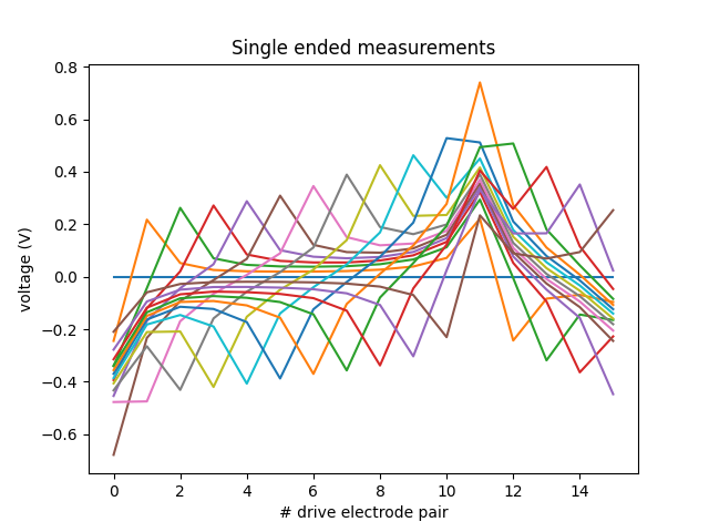
print(fem_res.v_eit(i_t=0,signed=True).shape)
plt.figure()
plt.plot(fem_res.v_eit(i_t=0,signed=True))

plt.xlabel("# drive electrode pair")
plt.ylabel("voltage (V)")
plt.title("Single ended measurements")
plt.figure()
plt.plot(inv_pb.fromat_data())
plt.xlabel("# drive electrode pair")
plt.ylabel("voltage (V)")
plt.title("Diferentrial measurements")
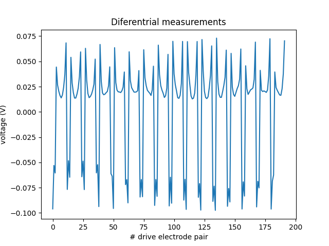
(16, 16)

Text(0.5, 1.0, 'Diferentrial measurements')
For this first tutorial, only one image will be generated at the peak of activity.
The reconstruction method used is dynamic, thus two sets of measurements are required:
When the fibres are at rest t=0 (
i_t=0).At the peak of activity t=t_max.
To find the index i_tmax, a simple method consists of examining res.dv_eit for one electrode over time and finding the time point where the absolute value is maximal, as done in the next cell.
_dv = fem_res.dv_eit(i_e=fem_res.n_e//2, i_p=0,)

i_tmax = np.argmax(np.abs(_dv))

print(f"t_max={fem_res["t"][i_tmax]}ms, (i_tmax={i_tmax})")


fig, ax = plt.subplots()
ax.plot(fem_res.t(), fem_res.dv_eit(i_e=fem_res.n_e//2, i_p=0), label=f"Voltage shift measured by E{int(fem_res.n_e//2)}")
ax.axvline(fem_res["t"][i_tmax], color=("r",.8), label="Measurment time used for\n the reconstruction")
ax.set_xlabel("time ($ms$)")
ax.set_ylabel("voltage ($V$)")
ax.legend()
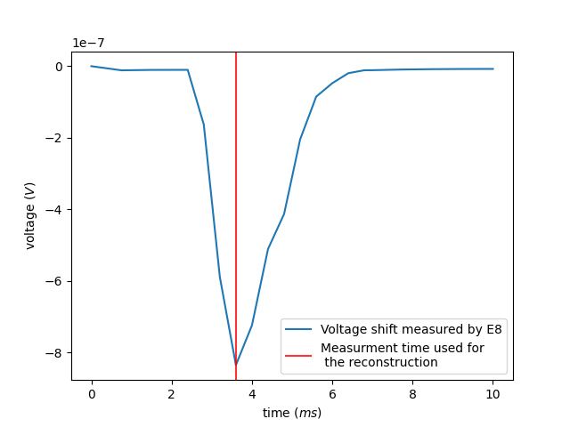
t_max=3.6000000000003696ms, (i_tmax=7)

<matplotlib.legend.Legend object at 0x707775a86570>
If required the data formatted for pyEIT solvers can be extracted using fromat_data as shown bellow:
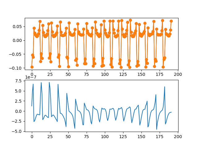
[<matplotlib.lines.Line2D object at 0x7077b7228380>]
Here is where the reconstruction is done.
To reconstruct the images from the measurements the mesh and scan protocol have to be initialized in Pyeit
Then the solver object is defined and used on the two sets of measurements.
ds = inv_pb.solve(i_t=i_tmax)[0]

print(type(ds), ds.shape, inv_pb.mesh_obj.node.shape, inv_pb.mesh_obj.element.shape)
<class 'numpy.ndarray'> (2821,) (1476, 3) (2821, 3)
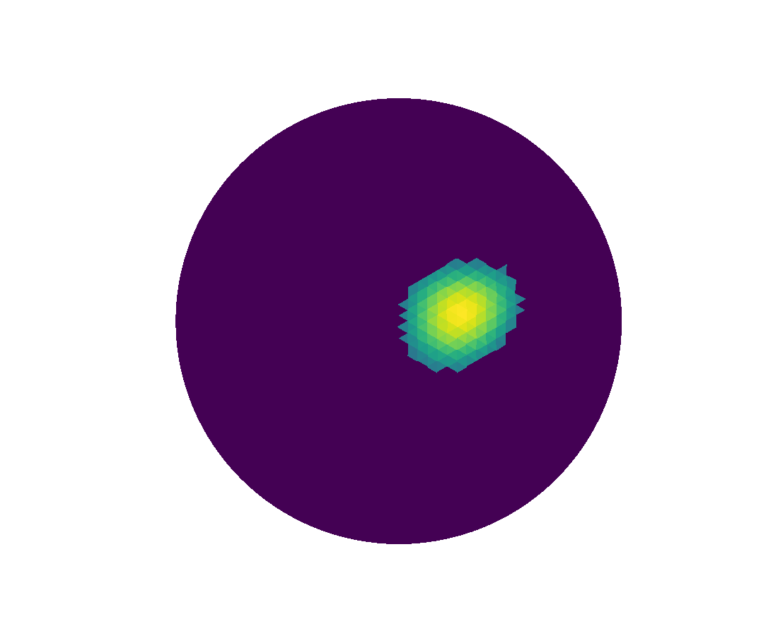
Finally, the reconstruction can be plotted with matplotlib as bellow:
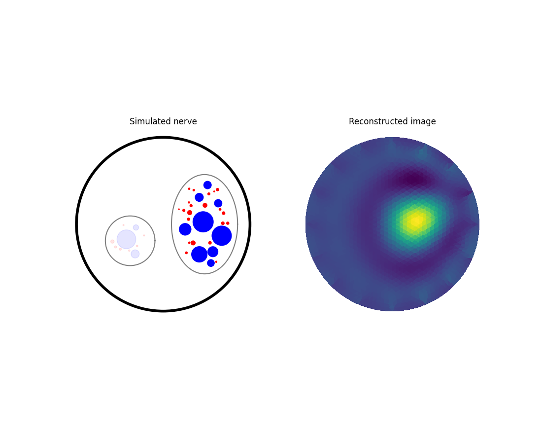
An additional filter can be applied when plotting the reconstructed image.
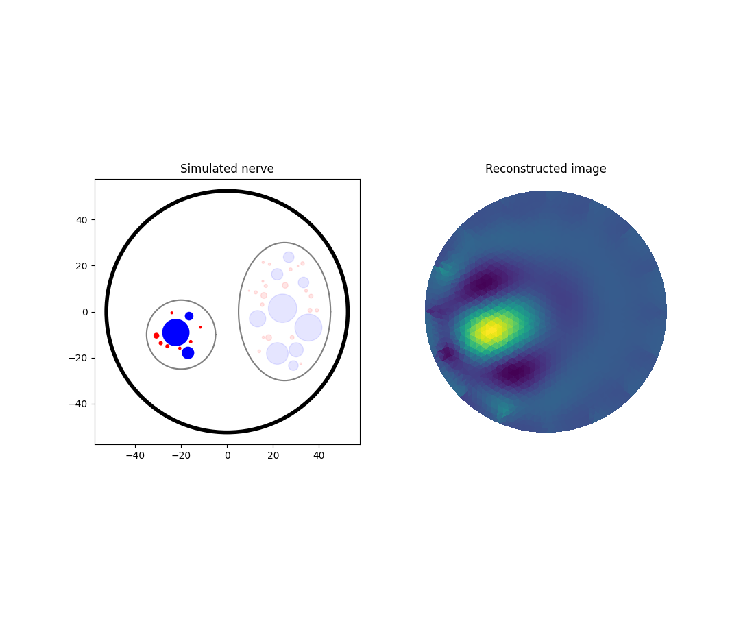
Second fascicle activation
To summarize more concisely, the same process can be repeated for activity generated only in the second (left) fascicle.
Forward problem
eit_instance = eit.EIT2DProblem(nerve_data, res_dname=res_dir, label=test_id, **parameters)

## Nerve simulation
sim_param = {"t_sim":t_sim}
nrn_res_2 = eit_instance.simulate_nerve(t_start=t_iclamp, sim_param=sim_param, fasc_list=[2])


## Impedance simulation
eit_instance._setup_problem()
# Build mesh
eit_instance.build_mesh()
# Simulate nerve
fem_res_2 = eit_instance.simulate_eit()
fascicle 1/2 -- 3 CPUs: 30 / 30 ━━━━━━━━━━━━━━━━━━━━━━━━━━━ 100% 0:00:00 0:01:14
fascicle 2/2 -- 3 CPUs: 10 / 10 ━━━━━━━━━━━━━━━━━━━━━━━━━━━ 100% 0:00:00 0:00:40
process 1 -- 3 : 112/112 ━━━━━━━━━━━━━━━━━━━━━━━━━━━━━━━━━━ 100% 0:00:00 0:00:38
process 2 -- 3 : 112/112 ━━━━━━━━━━━━━━━━━━━━━━━━━━━━━━━━━━ 100% 0:00:00 0:00:39
process 3 -- 3 : 112/112 ━━━━━━━━━━━━━━━━━━━━━━━━━━━━━━━━━━ 100% 0:00:00 0:00:38
Inverse problem
inv_pb_2 = eit.pyeit_inverse(data=fem_res_2)

ds = inv_pb_2.solve(i_t=i_tmax)[0]

# draw
fig, axs2 = plt.subplots(1, 2, figsize=(11, 9))
nrn_res_2.plot_recruited_fibers(axs2[0])

axs2[0].set_title("Simulated nerve")

inv_pb_2.plot(ax=axs2[1], i_t=i_tmax)
axs2[1].set_title("Reconstructed image")
axs2[1].set_aspect("equal", adjustable="box")
Final summary plot
# draw
fig, axs = plt.subplots(2, 3, figsize=(11, 9), layout="constrained")

nrn_res.plot_recruited_fibers(axs[0,0])
axs[0,0].set_axis_off()

inv_pb.plot(ax=axs[0,1], i_t=i_tmax)
axs[0,1].set_aspect("equal", adjustable="box")
inv_pb.plot(ax=axs[0,2], i_t=i_tmax, filter=eit.utils.thr_window)
axs[0,2].set_aspect("equal", adjustable="box")
nrn_res_2.plot_recruited_fibers(axs[1,0])
axs[1,0].set_axis_off()

inv_pb_2.plot(ax=axs[1,1], i_t=i_tmax)
axs[1,1].set_aspect("equal", adjustable="box")
inv_pb_2.plot(ax=axs[1,2], i_t=i_tmax, filter=eit.utils.thr_window)
axs[1,2].set_aspect("equal", adjustable="box")

axs[0,0].set_title("Simulated nerve")
axs[0,1].set_title("Reconstructed image")
axs[0,2].set_title("Filtered reconstruction")
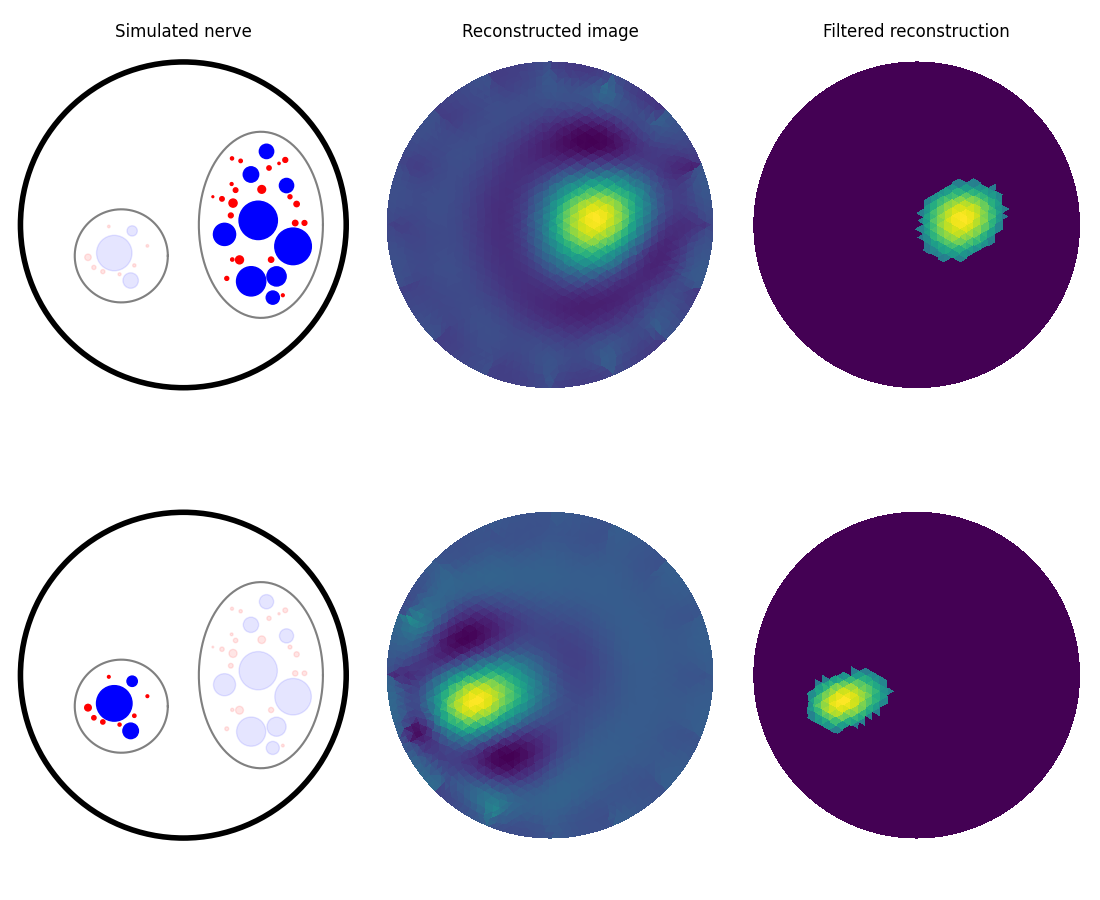
Text(0.5, 1.0, 'Filtered reconstruction')
Total running time of the script: (5 minutes 29.062 seconds)