Note
Go to the end to download the full example code.
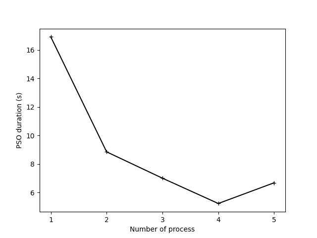
Optimization change number of processes
This example shows how to set the number of processes used for optimization. The exact same scenario from Tutorial 5 is used:
The objective is to minimize the energy required by a LIFE electrode to trigger a single myelinated fiber using a rectangular pulse stimulus.
Note
For optimization over parallelizable context (nerve or fascicle), the parallelization is done only for the context simulation
See also
See the Parallel computation and Optimization user guides.
best input vector: [3.8812254810415108, 0.21190886399270414]
best cost: 0.031922483533674786
best input vector: [3.8812254810415108, 0.21190886399270414]
best cost: 0.031922483533674786
best input vector: [3.8812254810415108, 0.21190886399270414]
best cost: 0.031922483533674786
best input vector: [3.8812254810415108, 0.21190886399270414]
best cost: 0.031922483533674786
best input vector: [3.8812254810415108, 0.21190886399270414]
best cost: 0.031922483533674786
import nrv
import matplotlib.pyplot as plt
import numpy as np
if __name__ == "__main__":
# -------------------------- #
# Cost function definition #
# -------------------------- #
my_cost0 = nrv.cost_function()
# Setting Static Context
ax_l = 10000 # um
ax_d=10
ax_y=50
ax_z=0
axon_1 = nrv.myelinated(L=ax_l, d=ax_d, y=ax_y, z=ax_z)
LIFE_stim0 = nrv.FEM_stimulation()
LIFE_stim0.reshape_nerve(Length=ax_l)
life_d = 25 # um
life_length = 1000 # um
life_x_0_offset = life_length/2
life_y_c_0 = 0
life_z_c_0 = 0
elec_0 = nrv.LIFE_electrode("LIFE", life_d, life_length, life_x_0_offset, life_y_c_0, life_z_c_0)
dummy_stim = nrv.stimulus()
dummy_stim.pulse(0, 0.1, 1)
LIFE_stim0.add_electrode(elec_0, dummy_stim)
axon_1.attach_extracellular_stimulation(LIFE_stim0)
axon_1.get_electrodes_footprints_on_axon()
static_context = axon_1.save(save=False, extracel_context=True)
del axon_1
t_sim = 5
dt = 0.005
kwarg_sim = {
"dt":dt,
"t_sim":t_sim,
}
my_cost0.set_static_context(static_context, **kwarg_sim)
# Setting Context Modifier
t_start = 1
I_max_abs = 100
cm_0 = nrv.biphasic_stimulus_CM(start=t_start, s_cathod="0", t_cathod="1", s_anod=0)
my_cost0.set_context_modifier(cm_0)
# Setting Cost Evaluation
costR = nrv.recrutement_count_CE(reverse=True)
costC = nrv.stim_energy_CE()
cost_evaluation = costR + 0.01 * costC
my_cost0.set_cost_evaluation(cost_evaluation)
# -------------------------- #
# PSO Optimizer definition #
# -------------------------- #
pso_kwargs = {
"maxiter" : 10,
# "maxiter" : 50,
"n_particles" : 10,
# "n_particles" : 20,
"opt_type" : "local",
"options": {'c1': 0.6, 'c2': 0.6, 'w': 0.8, 'k': 3, 'p': 1},
"bh_strategy": "reflective",
}
pso_opt = nrv.PSO_optimizer(**pso_kwargs)
t_end = 0.5
duration_bound = (0.01, t_end)
bounds0 = (
(0, I_max_abs),
duration_bound
)
pso_kwargs_pb_0 = {
"dimensions" : 2,
"bounds" : bounds0,
"comment":"pulse"}
n_proc_list = [1, 2, 3, 4, None]
best_res_list = []
duration_list = []
# Problem definition
fig_costs, axs_costs = plt.subplots(2, 1)
for n_proc in n_proc_list:
np.random.seed(444)
my_prob = nrv.Problem(n_proc=n_proc)
my_prob.costfunction = my_cost0
my_prob.optimizer = pso_opt
res0 = my_prob(**pso_kwargs_pb_0)
best_res_list += [res0["x"]]
duration_list += [res0["optimization_time"]]
print("best input vector:", res0["x"], "\nbest cost:", res0["best_cost"])
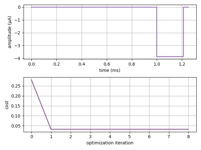
stim = cm_0(res0.x, static_context).extra_stim.stimuli[0]
stim.plot(axs_costs[0], label="rectangle pulse")
axs_costs[0].set_xlabel("best stimulus shape")
axs_costs[0].set_xlabel("time (ms)")
axs_costs[0].set_ylabel("amplitude (µA)")
axs_costs[0].grid()
res0.plot_cost_history(axs_costs[1])
axs_costs[1].set_xlabel("optimization iteration")
axs_costs[1].set_ylabel("cost")
axs_costs[1].grid()
fig_costs.tight_layout()
simres = res0.compute_best_pos(my_cost0)
simres.rasterize("V_mem")
del my_prob
plt.figure()
n_proc_list_int = [1, 2, 3, 4, 5]
n_proc_list_labs = [str(i) for i in n_proc_list_int]
n_proc_list_labs[-1] = "default = 3"
plt.plot(n_proc_list_int, duration_list, "-+k")
plt.xticks(n_proc_list_int, labels=n_proc_list_int)
plt.xlabel("Number of process")
plt.ylabel("PSO duration (s)")
plt.show()
Total running time of the script: (0 minutes 53.048 seconds)