Note

Go to the end to download the full example code.

Tutorial 5 - First optimization problem using NRV

In this tutorial, the optimization formalism used in NRV is illustrated through a detailed example.

First optimization: Pulse Stimulus on Single axon

The objective of the first optimization problem is to minimize a rectangle pulse stimulus energy required by a LIFE-electrode to trigger a single myelinated fibre.

Cost function

To begin, we can create an empty cost function object and fill it progressively with its components.

## Cost function definition
my_cost0 = nrv.cost_function()

Static context

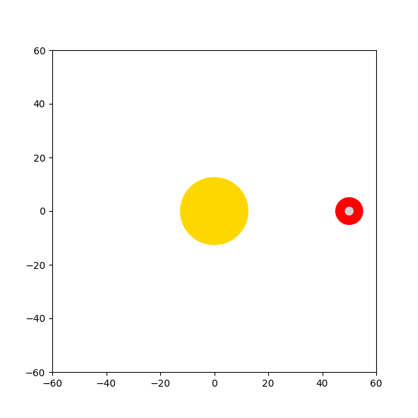
The first step to implement the optimization is to define the static context. This context can be generated with the following script, the same way as in previous Tutorials Tutorial 1. In this first example the context is only composed of:

a myelinated axon: \(10mm\) long, \(10\mu m\) diameter large, with a centre located at \((y=50\mu m, z=0)\)

a LIFE-electrode: \(1mm\) long, \(25\mu m\) diameter large, with a centre located at \((x=500\mu m, y=0, z=0)\)

Note

As the stimulus of the LIFE-electrode will be regenerated during the optimization a dummy stimulus is associated to the electrode

Note

To speed up the simulations done later, in the optimization, the footprints of the electrode on the axon are computed with get_electrodes_footprints_on_axon method and save with the context.

Once generated, the axon and its extracellular context can be saved in a .json file with using NRV save methods (save methods). This file will be loaded by the cost_function every times it will be called for the optimization.

ax_l = 10000 # um
ax_d=10
ax_y=50
ax_z=0
axon_1 = nrv.myelinated(L=ax_l, d=ax_d, y=ax_y, z=ax_z)


LIFE_stim0 = nrv.FEM_stimulation()
LIFE_stim0.reshape_nerve(Length=ax_l)
life_d = 25 # um
life_length = 1000 # um
life_x_0_offset = life_length/2
life_y_c_0 = 0
life_z_c_0 = 0
elec_0 = nrv.LIFE_electrode("LIFE", life_d, life_length, life_x_0_offset, life_y_c_0, life_z_c_0)

dummy_stim = nrv.stimulus()
dummy_stim.pulse(0, 0.1, 1)
LIFE_stim0.add_electrode(elec_0, dummy_stim)

axon_1.attach_extracellular_stimulation(LIFE_stim0)
axon_1.get_electrodes_footprints_on_axon()
axon_dict = axon_1.save(extracel_context=True)

fig, ax = plt.subplots(1, 1, figsize=(6,6))
axon_1.plot(ax)
ax.set_xlim((-1.2*ax_y, 1.2*ax_y))
ax.set_ylim((-1.2*ax_y, 1.2*ax_y))

del axon_1

Once this static context has been saved in the cost function it should be linked with the cost_function.

For that purpose, we can use the method set_static_context as bellow.

Note that additional keys arguments can be added to precise simulation parameter. Here we impose a simulation time of \(5ms\) and a time step of \(5\mu s\). These arguments will be added when the simulate method will be called so all the parameters of a standard simulation can be as in previous example

static_context = axon_dict
t_sim = 5
dt = 0.005
kwarg_sim = {
    "dt":dt,
    "t_sim":t_sim,
}

my_cost0.set_static_context(static_context, **kwarg_sim)

Context modifier

The next step is to define how to interpret the tuning parameters to modify the static context. In our problem, we want to modify the LIFE-electrode’s stimulus shape and evaluate its impact on the fiber. There are countless ways to define a waveform from a set of points, so let’s consider a very simple method:

The stimulus is a cathodic conventional square pulse. In this scenario, both the pulse duration \(T_{sq}\) and pulse amplitude \(I_{sq}\) can be optimized, resulting in a two-dimensional optimization problem. The tuning parameters input vector \(\mathcal{X}_{sq}\) of the optimization problem is thus defined as follows:

\[\mathcal{X}_{sq} = \begin{pmatrix} I_{sq} & T_{sq} \end{pmatrix} \;\]

Implementation:

In NRV, the modification of the static context can either be done with a callable class or a function. Some context_modifier classes have already been implemented in NRV.

The biphasic_stimulus_CM is appropriate for our problem. Such simulable add a biphasic pulse to a given electrode of a nrv_simulable object. To fit with our problem, we set the following arguments:

start=1: the cathodic pulse to start at \(1ms\).

s_cathod=”0” the cathodic pulse amplitude is defined by the first value of the input vector \(\mathcal{X}_{sq}\).

T_cathod=”1” the cathodic pulse duration is defined by the second value of the input vector \(\mathcal{X}_{sq}\).

s_anod=0 anodic pulse amplitude is 0 (we consider a monophasic pulse).

Note

Arguments of biphasic_stimulus_CM are similar to those of biphasic_pulse(). User can either set the argument to a specific value or specify that it should be defined by a tuning parameters input vector. In the second case the argument should be a str of the index of the argument in the vector.

t_start = 1
I_max_abs = 100

cm_0 = nrv.biphasic_stimulus_CM(start=t_start, s_cathod="0", t_cathod="1", s_anod=0)
my_cost0.set_context_modifier(cm_0)

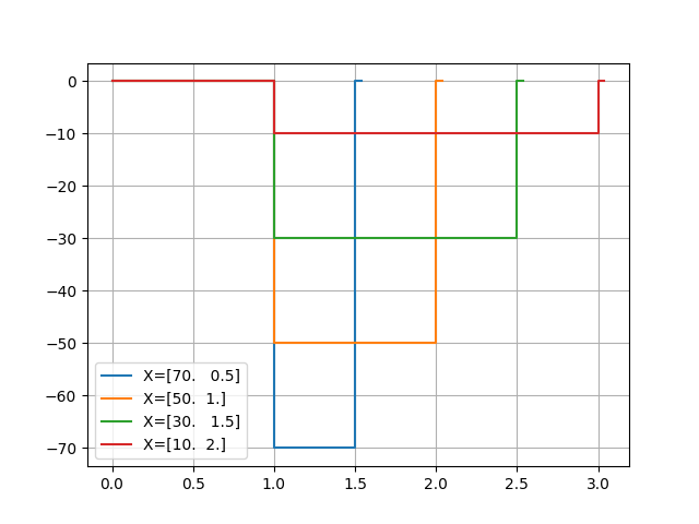
The following lines illustrate the stimuli generated by the cm_0 for various input parameters.

As expected:

The first dimension sets the pulse’s negative amplitude.
The second sets the pulse duration.

test_points = np.array([[70, 0.5], [50, 1], [30, 1.5], [10, 2]])

fig, ax = plt.subplots()
ax.grid()
for X in test_points:
    axon_x = cm_0(X, static_context)
    stim = axon_x.extra_stim.stimuli[0]
    stim.plot(ax, label=f"X={X}")
    ax.legend()
    del axon_x

Cost Evaluation

In our problem, we want at the same time to minimize the energy of the stimulus and maximize the number of fibre recruited. Therefore, we can evaluate the cost of a stimulus on the context using the following equation:

\[Cost = \alpha_e\sum_{t_k}(i_{stim}^2(t_k))+\alpha_r(N_{axon}-N_{recruited})\]

With:

\(t_k\) as the discrete time step of the simulation.
\(N_{axon}\) as the number of axon simulated, 1 in this first problem.
\(N_{recruited}\) as the number of fibre triggered by the stimulation.
\(\alpha_e\) and \(\alpha_r\) as two weighting coefficients.

Implementation:

In NRV, the computation of this cost from simulation results is handled by a function or a callable class instance called cost_evaluation. As for context_modifier, several cost_evaluation classes are already implemented in the NRV package. These classes can be combined with algebraic operations to easily generate more complex cases.

Here, the cost evaluation is generated using two classes implemented in NRV:

recrutement_count_CE: computes the number of triggered fibres.
stim_energy_CE: computes a value proportional to the stimulus energy.

# .. note::
#     The second term of the equation (`\alpha_r(N_{axon} - N_{recruited})`) essentially represents a function that is 1 if the fibre is triggered and 0 otherwise. This seemingly complicated notation allows us to use the same equation to evaluate a stimulus in contexts involving a larger number of axons.

# .. note::
#     With a good knowledge of the simulation results, it is possible to implement custom `cost_evaluation`, similar to `context_modifier`.
#   It should be a function or a callable class taking a `sim_results` object and any additional `kwargs` parameters, returning a corresponding cost (`float`).

costR = nrv.recrutement_count_CE(reverse=True)
costC = nrv.stim_energy_CE()

cost_evaluation = costR + 0.01 * costC
my_cost0.set_cost_evaluation(cost_evaluation)

Optimization problem

At this point, the cost function that should be minimized is fully defined. We can now proceed to define the entire optimization process by selecting the appropriate optimizer.

The cost function defined for this problem is not continuous due to the second term of the cost evaluation equation (alpha_r(N_{axon} - N_{recruited})). Therefore, a meta-heuristic approach is more suitable for our needs.

We can thus instantiate a nrv.optim.PSO_optimizer object adapted to our problem as bellow. The parameters relative to the optimization are added at the instantiation. Here:

maxiter: sets the number of iterations of the optimization.

n_particles: set the number of particle of the swarm.

opt_type: sets the neighbour topology as star (when “global”) or ring (when “local”).

options: sets the Pyswarms’s PSO option.

bh_strategy: sets the out-of-bounds handling strategy.

See Pyswarms documentation for more information

pso_kwargs = {
    "maxiter" : 50,
    "n_particles" : 20,
    "opt_type" : "local",
    "options": {'c1': 0.6, 'c2': 0.6, 'w': 0.8, 'k': 3, 'p': 1},
    "bh_strategy": "reflective",
}
pso_opt = nrv.PSO_optimizer(**pso_kwargs)

Once both the cost_function and the optimizer are defined the optimization problem can be simply as bellow

# Problem definition
my_prob = nrv.Problem()
my_prob.costfunction = my_cost0
my_prob.optimizer = pso_opt

By calling this optimizer we can the run the optimization. Additional parameters can be set at this time using key arguments. Here, we use this option to set the PSO parameters relative to this problem:

dimensions: dimension of the input vector

bounds: boundaries of each dimension of the input vector

comment: optional str comment which will be added to the results dictionary

An optim_results instance will be returned from the optimization containing all results and parameters of the optimization.

Note

The keys to used to parametrize the optimizer are the same as for instantiating the PSO_optimizer.

Note

As optim_results class inherit from nrv_result, all results can either be access as dictionary keys or as class attributes and post-processing built-in method can be used

t_end = 0.5
duration_bound = (0.01, t_end)
bounds0 = (
    (0, I_max_abs),
    duration_bound
)
pso_kwargs_pb_0 = {
    "dimensions" : 2,
    "bounds" : bounds0,
    "comment":"pulse"}

res0 = my_prob(**pso_kwargs_pb_0)

Hurray! The first optimization is now complete.

We can check the best input vector and the best final cost stored in res0[“x”] and res0[“best_cost”] respectively.

print("best input vector:", res0["x"], "\nbest cost:", res0["best_cost"])

best input vector: [3.99748583236465, 0.18451328349588564]
best cost: 0.029485327795478525

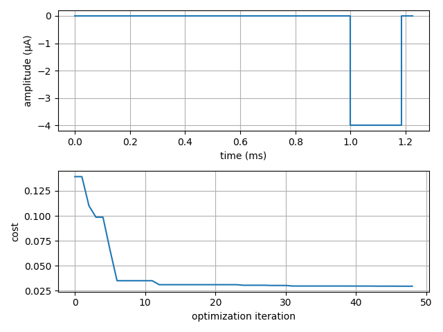
We can explore further the results of the optimization by plotting the best stimulus shape and the cost history.

fig_costs, axs_costs = plt.subplots(2, 1)

stim = cm_0(res0.x, static_context).extra_stim.stimuli[0]
stim.plot(axs_costs[0], label="rectangle pulse")
axs_costs[0].set_xlabel("best stimulus shape")
axs_costs[0].set_xlabel("time (ms)")
axs_costs[0].set_ylabel("amplitude (µA)")
axs_costs[0].grid()

res0.plot_cost_history(axs_costs[1])
axs_costs[1].set_xlabel("optimization iteration")
axs_costs[1].set_ylabel("cost")
axs_costs[1].grid()
fig_costs.tight_layout()

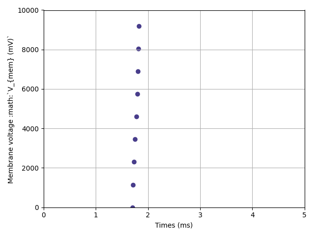
Using the method compute_best_pos, the axon with the optimized stimulus can be simulated.

This can be useful to make sure the axon is activated by plotting the rasterized \(V_{mem}\) as in Tutorial 1.

simres = res0.compute_best_pos(my_cost0)
simres.rasterize("V_mem")
plt.figure()
plt.scatter(simres["V_mem_raster_time"], simres["V_mem_raster_x_position"], color='darkslateblue')
plt.xlabel('Times (ms)')
plt.ylabel('Membrane voltage :math:`V_{mem} (mV)`')
plt.xlim(0, t_sim)
plt.ylim(0, simres["L"])
plt.grid()
plt.tight_layout()

Second optimization spline interpolated stimulus

At this point, we have found a rectangle pulse stimulus shape triggering our fibre with a minimal energy. Let’s see if we can find a better cost with a more complex stimulus shape.

In this new problem, we can define the stimulus as a cathodic pulse through interpolated splines over \(2\) points which are individually defined in time and amplitude. This second optimization scenario results in a \(4\)-dimensional problem with the input vector \(\mathcal{X}_{s_2}\) defined as:

\[\mathcal{X}_{s_2} = \begin{pmatrix} I_{s_1} & t_{s_1} & I_{s_2} & t_{s_2} \end{pmatrix}\]

With \(I_{s_1}\) and \(t_{s_1}\) the amplitude and time of the first point and \(I_{s_2}\) and \(t_{s_2}\) those of the second.

As in the first optimization, the stimulus generation from input vector is handled by the context_modifier. So let’s define a new one which will fit our purpose. This can be done using another built-in class in NRV: biphasic_stimulus_CM(). To fit with our problem the following parameters are set

kwrgs_interp = {
    "dt": dt,
    "amp_start": 0,
    "amp_stop": 0,
    "intertype": "Spline",
    "bounds": (-I_max_abs, 0),
    "t_sim":t_sim,
    "t_end": t_end,
    "t_shift": t_start,
    }
cm_1 = nrv.stimulus_CM(interpolator=nrv.interpolate_Npts, intrep_kwargs=kwrgs_interp, t_sim=t_sim)

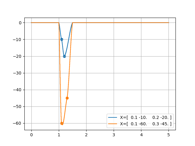
As before, we can plot several stimulus shapes generated from this new context_modifier

test_points = np.array([[.1, -10, .2, -20], [.1, -60, .3, -45]])

fig, ax = plt.subplots()
ax.grid()
for X in test_points:
    axon_x = cm_1(X, static_context)
    stim = axon_x.extra_stim.stimuli[0]
    stim.plot(ax, label=f"X={X}")
    plt.scatter(t_start+X[::2], X[1::2])
    ax.legend()
    del axon_x

This time all the components of the new cost_function are already defined. It can thus be directly defined at the instantiation of the cost_function as bellow.

my_cost_1 = nrv.cost_function(
    static_context=static_context,
    context_modifier=cm_1,
    cost_evaluation=cost_evaluation,
    kwargs_S=kwarg_sim)

We can now update our optimization problem with this second cost_function.

Since the number of dimensions and the bounds of each dimension are different from the first problem, the optimizer parameters must also be updated. This can be done when running the optimization.

my_prob.costfunction = my_cost_1

I_bound = (-I_max_abs, 0)
t_bound = (0, t_end)
bounds1 = (t_bound, I_bound, t_bound, I_bound)
pso_kwargs_pb_1 = {
    "dimensions" : 4,
    "bounds" : bounds1,
    "comment":"spline",
}

res1 = my_prob(**pso_kwargs_pb_1)

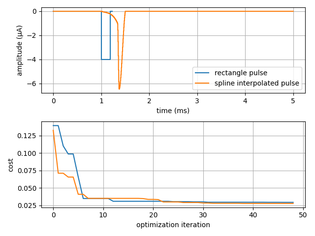
Finally, we can update the figure of the first results with this new optimized stimulus and the cost history to compare the results.

fig_costs, axs_costs = plt.subplots(2, 1)

stim_0 = cm_0(res0.x, static_context).extra_stim.stimuli[0]
stim_1 = cm_1(res1.x, static_context).extra_stim.stimuli[0]

stim_0.plot(axs_costs[0], label="rectangle pulse")
stim_1.plot(axs_costs[0], label="spline interpolated pulse")
axs_costs[0].set_xlabel("best stimulus shape")
axs_costs[0].set_xlabel("time (ms)")
axs_costs[0].set_ylabel("amplitude (µA)")
axs_costs[0].grid()
axs_costs[0].legend()

res0.plot_cost_history(axs_costs[1])
res1.plot_cost_history(axs_costs[1])
axs_costs[1].set_xlabel("optimization iteration")
axs_costs[1].set_ylabel("cost")
axs_costs[1].grid()
fig_costs.tight_layout()

Total running time of the script: (3 minutes 48.545 seconds)