Combining Stimuli in NRV

This example shows how logical and arithmetical operations on NRV’s stimulus object can facilitate the creation of complex stimulus.

import nrv
import matplotlib.pyplot as plt
from numpy import exp


if __name__ == '__main__':
    #####################################
    # Example of combination of stimuli #
    #####################################
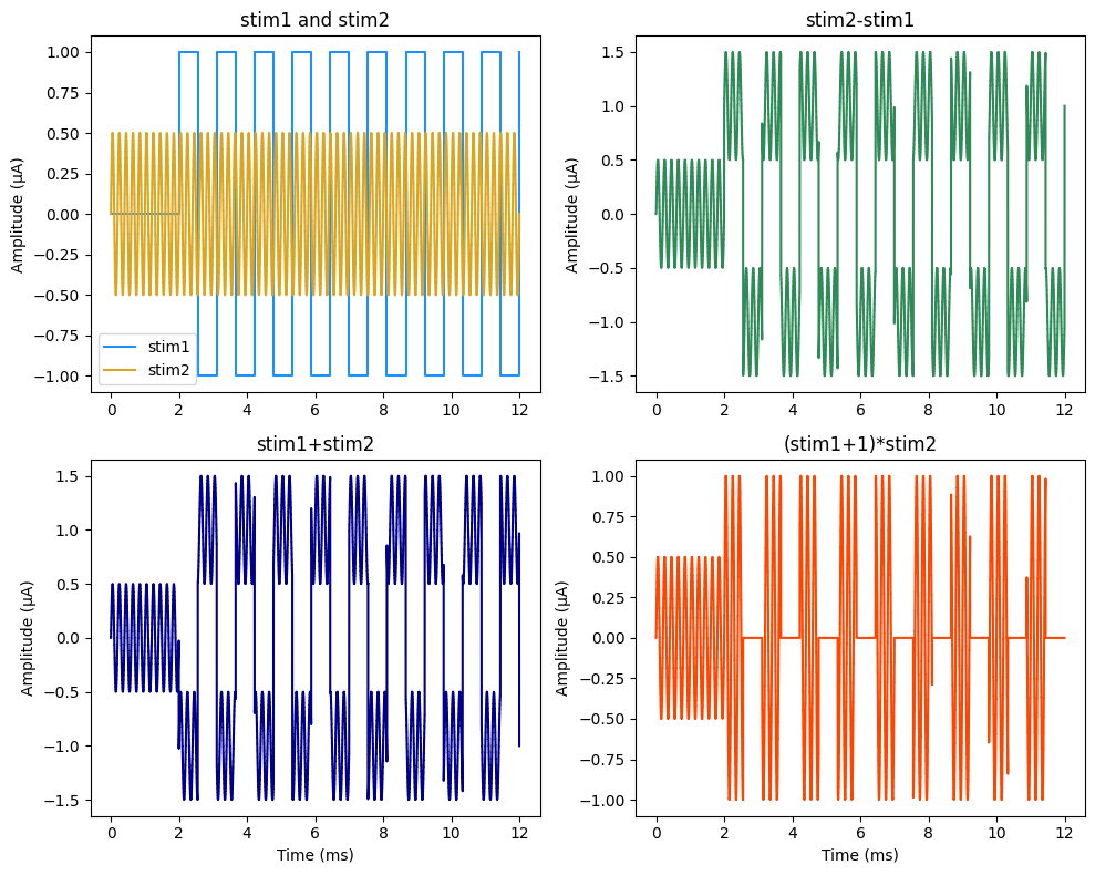
    stim1, stim2 = nrv.stimulus(), nrv.stimulus()

    # stim1 parameters
    t_start = 2
    duration = 10
    amp1 = 1
    f_stim1 = 1
    stim1.square(t_start, duration, amp1, f_stim1, 0, 0.5)
    # stim2 parameters
    f_stim2 = 5
    amp2 = 0.5
    stim2.sinus(0, t_start+duration, amp2, f_stim2)

    # computations with +,-,*
    stim3 = stim1 + stim2
    stim4 = stim2 - stim1
    stim5 = (stim1 + 1) * stim2

    #print(dir(biphasic_stim))

    fig, axs = plt.subplots(2, 2, layout='constrained', figsize=(10, 8))
    stim1.plot(axs[0,0], label='stim1',color = "dodgerblue")
    stim2.plot(axs[0,0], label='stim2',color = "goldenrod")
    stim3.plot(axs[0,1], label='stim1+stim2',color = "seagreen")
    stim4.plot(axs[1,0], label='stim2-stim1',color = "darkblue")
    stim5.plot(axs[1,1], label='(stim1+1)*stim2',color = "orangered")

    axs[0,0].legend()
    axs[0,0].set_title("stim1 and stim2")
    axs[1,0].set_title("stim1+stim2")
    axs[0,1].set_title("stim2-stim1")
    axs[1,1].set_title("(stim1+1)*stim2")

    axs[0,0].set_ylabel('Amplitude (µA)')
    axs[0,1].set_ylabel('Amplitude (µA)')
    axs[1,0].set_ylabel('Amplitude (µA)')
    axs[1,1].set_ylabel('Amplitude (µA)')

    axs[1,0].set_xlabel('Time (ms)')
    axs[1,1].set_xlabel('Time (ms)')
    fig.tight_layout()

###################################
# Example of amplitude modulation #
###################################
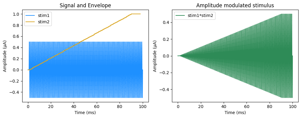
if __name__ == '__main__':
    stim1, stim2 = nrv.stimulus(), nrv.stimulus()

    f_stim = 1
    t_start = 1
    duration = 99
    amp = 0.5

    t_ramp_stop = 90
    amp_start = 0
    amp_max = 1

    stim1.sinus(t_start, duration, amp, f_stim)
    stim2.ramp_lim(t_start, t_ramp_stop, amp_start, amp_max, duration, dt=1)

    stim3 = stim1*stim2
    fig, axs = plt.subplots(1, 2, layout='constrained', figsize=(10, 4))

    stim1.plot(axs[0],label = 'stim1',color = "dodgerblue")
    stim2.plot(axs[0],label = 'stim2',color = "goldenrod")

    axs[0].set_title('Signal and Envelope')
    stim3.plot(axs[1],label = 'stim1*stim2',color = "seagreen")
    axs[1].set_title('Amplitude modulated stimulus')

    axs[0].set_xlabel('Time (ms)')
    axs[0].set_ylabel('Amplitude (µA)')
    axs[1].set_xlabel('Time (ms)')
    axs[1].set_ylabel('Amplitude (µA)')
    axs[0].legend()
    axs[1].legend()
    fig.tight_layout()

#################################################
## Example of a complex custom stimulus design ##
##                                             ##
## simple pulse with a prepulse and charge     ##
## balance                                     ##
## modulation with a gaussian of borst of 10   ##
## patterns                                    ##
## repetition of the bursts                    ##
#################################################

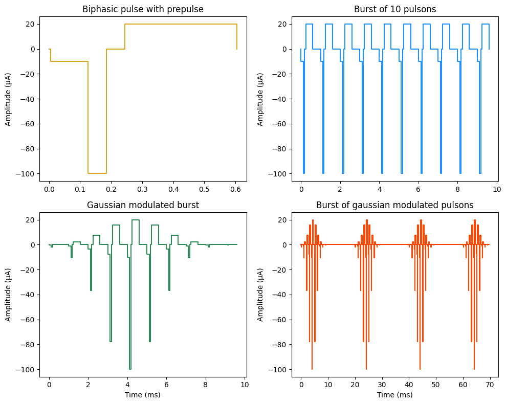
if __name__ == '__main__':
    start = 5e-3
    fig, axs = plt.subplots(2, 2, layout='constrained', figsize=(10, 8))

    # waveform parameters
    complex_stim = nrv.stimulus()
    prepulse_amp = -10              # in uA
    t_prepulse = 120e-3             # in ms
    cath_amp = -100                 # in uA
    t_cath = 60e-3                  # in ms
    deadtime = 60e-3                # in ms
    an_amp = 20                     # in uA
    # prepulse and cathodic pulse
    complex_stim.pulse(start, prepulse_amp)
    complex_stim.pulse(start + t_prepulse, cath_amp, t_cath)
    complex_stim.s[-1] = 0
    # compute the balancing time and anodic pulse
    an_duration = abs(prepulse_amp*t_prepulse + cath_amp*t_cath)/an_amp
    complex_stim.pulse(complex_stim.t[-1] + deadtime, an_amp, an_duration)
    # plot the pattern
    complex_stim.plot(axs[0, 0],color = "goldenrod")
    axs[0, 0].set_title('Biphasic pulse with prepulse')
    #axs[0, 0].set_xlabel('Time (ms)')
    axs[0, 0].set_ylabel('Amplitude (µA)')

    # create burst of 10 patterns
    freq = 1.                       # in kHz
    # finish the period
    t_blank = 1/freq - (start + t_prepulse + t_cath + deadtime + an_duration)
    N_patterns = 10
    s_pattern, t_pattern = complex_stim.s, complex_stim.t
    for i in range(N_patterns-1):
        complex_stim.concatenate(s_pattern, t_pattern, t_shift=t_blank)
    # plot the pattern
    complex_stim.plot(axs[0, 1],color = "dodgerblue")
    axs[0, 1].set_title('Burst of 10 pulsons')
    #axs[0, 1].set_xlabel('Time (ms)')
    axs[0, 1].set_ylabel('Amplitude (µA)')

    # modulate with gaussian envelope
    def my_gaussian(t, f, N_patterns):
        return exp(-((t - ((N_patterns/2)-1)*(1/f))**2)/4)


    envelope = nrv.stimulus()
    for k in range(N_patterns):
        envelope.pulse(k*(1/freq), my_gaussian(k*(1/freq), freq, N_patterns))

    modulated_pattern = complex_stim * envelope
    modulated_pattern.plot(axs[1,0],color = "seagreen")
    axs[1, 0].set_title('Gaussian modulated burst')
    axs[1, 0].set_xlabel('Time (ms)')
    axs[1, 0].set_ylabel('Amplitude (µA)')

    # construct repeted groups of burst
    N_burst = 4
    f_burst = 0.05
    s_burst, t_burst = modulated_pattern.s, modulated_pattern.t
    t_blank = 1/f_burst - modulated_pattern.t[-1]
    for i in range(N_burst-1):
        modulated_pattern.concatenate(s_burst, t_burst, t_shift=t_blank)
    modulated_pattern.plot(axs[1,1],color ="orangered")
    axs[1, 1].set_title('Burst of gaussian modulated pulsons')
    axs[1, 1].set_xlabel('Time (ms)')
    axs[1, 1].set_ylabel('Amplitude (µA)')
    fig.tight_layout()

    #plt.show()