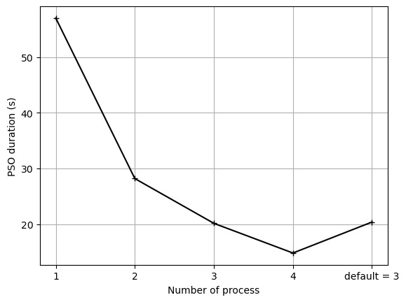
Optimization change number of processes

This example shows how to set the number of processes used for optimization. The exact same scenario from Tutorial 5 is used:

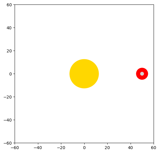
The objective is to minimize the energy required by a LIFE electrode to trigger a single myelinated fiber using a rectangular pulse stimulus.

Note

For optimization over parallelizable context (nerve or fascicle), the parallelization is done only for the context simulation

See also

Parallel computation and Optimization users’ guides.

import sys
sys.path.append("../../../")     #data path
import nrv

import matplotlib.pyplot as plt
import numpy as np
import os

N_test = "227"
figdir = f"./unitary_tests/figures/{N_test}_"

res_dir = f"./Example_/{N_test}"

# -------------------------- #
#  Cost function definition  #
# -------------------------- #
my_cost0 = nrv.cost_function()


# Setting Static Context
axon_file = res_dir + "myelinated_axon.json"

ax_l = 10000 # um
ax_d=10
ax_y=50
ax_z=0
axon_1 = nrv.myelinated(L=ax_l, d=ax_d, y=ax_y, z=ax_z)


LIFE_stim0 = nrv.FEM_stimulation()
LIFE_stim0.reshape_nerve(Length=ax_l)
life_d = 25 # um
life_length = 1000 # um
life_x_0_offset = life_length/2
life_y_c_0 = 0
life_z_c_0 = 0
elec_0 = nrv.LIFE_electrode("LIFE", life_d, life_length, life_x_0_offset, life_y_c_0, life_z_c_0)

dummy_stim = nrv.stimulus()
dummy_stim.pulse(0, 0.1, 1)
LIFE_stim0.add_electrode(elec_0, dummy_stim)

axon_1.attach_extracellular_stimulation(LIFE_stim0)
axon_1.get_electrodes_footprints_on_axon()
axon_dict = axon_1.save(save=False, fname=axon_file, extracel_context=True)

fig, ax = plt.subplots(1, 1, figsize=(6,6))
axon_1.plot(ax)
ax.set_xlim((-1.2*ax_y, 1.2*ax_y))
ax.set_ylim((-1.2*ax_y, 1.2*ax_y))

del axon_1

static_context = axon_dict
t_sim = 5
dt = 0.005
kwarg_sim = {
    "dt":dt,
    "t_sim":t_sim,
}

my_cost0.set_static_context(static_context, **kwarg_sim)

# Setting Context Modifier
t_start = 1
I_max_abs = 100
cm_0 = nrv.biphasic_stimulus_CM(start=t_start, s_cathod="0", t_cathod="1", s_anod=0)
my_cost0.set_context_modifier(cm_0)

# Setting Cost Evaluation
costR = nrv.recrutement_count_CE(reverse=True)
costC = nrv.stim_energy_CE()
cost_evaluation = costR + 0.01 * costC
my_cost0.set_cost_evaluation(cost_evaluation)


# -------------------------- #
#  PSO Optimizer definition  #
# -------------------------- #
pso_kwargs = {
    "maxiter" : 50,
    "n_particles" : 20,
    "opt_type" : "local",
    "options": {'c1': 0.6, 'c2': 0.6, 'w': 0.8, 'k': 3, 'p': 1},
    "bh_strategy": "reflective",
}
pso_opt = nrv.PSO_optimizer(**pso_kwargs)

t_end = 0.5
duration_bound = (0.01, t_end)
bounds0 = (
    (0, I_max_abs),
    duration_bound
)
pso_kwargs_pb_0 = {
    "dimensions" : 2,
    "bounds" : bounds0,
    "comment":"pulse"}


n_proc_list = [1, 2, 3, 4, None]
best_res_list = []
duration_list = []
# Problem definition
fig_costs, axs_costs = plt.subplots(2, 1)

for n_proc in n_proc_list:
    np.random.seed(444)
    my_prob = nrv.Problem(n_proc=n_proc)
    my_prob.costfunction = my_cost0
    my_prob.optimizer = pso_opt
    res0 = my_prob(**pso_kwargs_pb_0)
    best_res_list += [res0["x"]]
    duration_list += [res0["optimization_time"]]


    print("best input vector:", res0["x"], "\nbest cost:", res0["best_cost"])


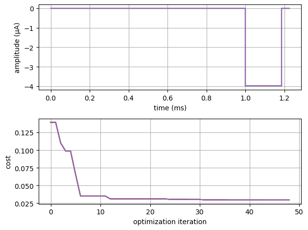
    stim = cm_0(res0.x, static_context).extra_stim.stimuli[0]
    stim.plot(axs_costs[0], label="rectangle pulse")
    axs_costs[0].set_xlabel("best stimulus shape")
    axs_costs[0].set_xlabel("time (ms)")
    axs_costs[0].set_ylabel("amplitude (µA)")
    axs_costs[0].grid()

    res0.plot_cost_history(axs_costs[1])
    axs_costs[1].set_xlabel("optimization iteration")
    axs_costs[1].set_ylabel("cost")
    axs_costs[1].grid()
    fig_costs.tight_layout()

    simres = res0.compute_best_pos(my_cost0)
    simres.rasterize("V_mem")
    del my_prob

NRV INFO: Mesh properties:
NRV INFO: Number of processes : 3
NRV INFO: Number of entities : 36
NRV INFO: Number of nodes : 11390
NRV INFO: Number of elements : 80986
NRV INFO: Static/Quasi-Static electrical current problem
NRV INFO: FEN4NRV: setup the bilinear form
NRV INFO: FEN4NRV: setup the linear form
NRV INFO: Static/Quasi-Static electrical current problem
NRV INFO: FEN4NRV: solving electrical potential
NRV INFO: FEN4NRV: solved in 4.018976449966431 s

PSO optimizer - 1 proc: 100%|██████████|50/50, best_cost=0.0295

best input vector: [3.989542355705061, 0.1852817779181298]
best cost: 0.029493916445033925

PSO optimizer - 2 procs: 100%|██████████|50/50, best_cost=0.0295

best input vector: [3.989542355705061, 0.1852817779181298]
best cost: 0.029493916445033925

PSO optimizer - 3 procs: 100%|██████████|50/50, best_cost=0.0295

best input vector: [3.989542355705061, 0.1852817779181298]
best cost: 0.029493916445033925

PSO optimizer - 4 procs: 100%|██████████|50/50, best_cost=0.0295

best input vector: [3.989542355705061, 0.1852817779181298]
best cost: 0.029493916445033925

PSO optimizer - 3 procs: 100%|██████████|50/50, best_cost=0.0295

best input vector: [3.989542355705061, 0.1852817779181298]
best cost: 0.029493916445033925

plt.figure()
n_proc_list_int = [1, 2, 3, 4, 5]
n_proc_list_labs = [str(i) for i in n_proc_list_int]
n_proc_list_labs[-1] = f"default = {nrv.parameters.optim_Ncores}"

plt.plot(n_proc_list_int, duration_list, "-+k")
plt.xticks(n_proc_list_int, labels=n_proc_list_labs)
plt.xlabel("Number of process")
plt.ylabel("PSO duration (s)")
plt.grid()