Note
Go to the end to download the full example code.
Tutorial 2 - Evaluation of propagation velocity with NRV
The presence of the myelin sheath on large axonal fibers transforms the so-called continuous conduction of unmyelinated fibers into a saltatory conduction, largely increasing the speed of action potential propagations. In this tutorial, we will simulated several myelinated and unmyelinated fiber model using NRV and investigate how it effects the action potential propagation speed.
First the nrv package is imported as well as the matplotlib
package used for plotting nrv’s simulation outputs. We will also use
some numpy’s function.
import numpy as np
import matplotlib.pyplot as plt
import nrv
Measuring Propagation Velocity of an unmyelinated fibers
First let’s create an unmyelinated object and specify the (y,z)
coordinates, diameter, length, and computationnal model used. The HH
model (Hodgkin and Huxley, 1952) is used here for the example.
The unmyelinated fiber is stimulated with an intracellular current clamp
that is attach to the fiber using the insert_I_Clamp method. The
generated AP will be used to measure the propagation speed.
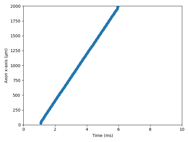
Axon is simulated and the simulated membrane’s voltage is rasterize to
facilitate the spike detection. For that, the rasterize method of the results object. The function detects the
presence of AP in the fiber across time and space using a threshold function.
We can plot the rasterized result to verify that an AP is indeed propagating through the fiber.
results.rasterize("V_mem")
fig, ax = plt.subplots(1)
results.raster_plot(ax,'V_mem')
ax.set_ylabel("Axon x-axis (µm)")
ax.set_xlabel("Time (ms)")
ax.set_xlim(0,results.tstop)
ax.set_ylim(0,np.max(results.x_rec))
fig.tight_layout()
The velocity of the propagating AP can be simply evaluated with the
built-in method get_avg_AP_speed of the results dictionary.
unmyelinated_speed = results.get_avg_AP_speed()
print(unmyelinated_speed)          #in m/s
0.406
Measuring Propagation Velocity of a myelinated fibers.
Those steps can be repeated but with a myelinated fiber model. Note that we defined a fixed number of nodes-of-ranvier and derived the length of the fiber from this number, rather than specifying its length directly.
## Axon creation
y = 0                                 # axon y position, in [um]
z = 0                                 # axon z position, in [um]
d = 10                                # axon diameter, in [um]
L = nrv.get_length_from_nodes(d, 21)  #Axon length is 21 node of Ranvier
model = "MRG"
axon = nrv.myelinated(y, z, d, L, model=model)

## test pulse
t_start = 1
duration = 0.1
amplitude = 5
axon.insert_I_Clamp(0, t_start, duration, amplitude)
t_sim = 5

## Simulation
results = axon(t_sim=t_sim)

results.rasterize("V_mem")
myelinated_speed = results.get_avg_AP_speed()
print(myelinated_speed)
65.094
As expected, the AP propagation is much faster in a large myelinated axon than small unmyelinated one!
# ## Velocity-diameter relationship

# The velocity of AP propagation in a fiber increases with its diameter.
# Let’s verify this with NRV and plot the propagation velocity diameter
# relationship for unmyelinated fibers. This typically takes less than 30s to calculate.

unmyelinated_diameters = np.linspace(0.1, 2, 10)            #10 unmyelinated fibers with diameter ranging from 0.1µm to 2µm.
unmyelinated_speed = []                                     #Empty list to store results

## Axon fixed parameters
y = 0
z = 0
L = 5000
model = "HH"

## test pulse fixed parameters
t_start = 1
duration = 0.1
amplitude = 5

t_sim = 10
for d in unmyelinated_diameters:

    #Axon creation
    axon1 = nrv.unmyelinated(y, z, d, L, model=model)
    axon1.insert_I_Clamp(0, t_start, duration, amplitude)

    ## Simulation
    results = axon1(t_sim=t_sim)
    del axon1

    results.rasterize("V_mem")
    unmyelinated_speed += [results.get_avg_AP_speed()]

#Plot the results
fig, ax  = plt.subplots()
ax.plot(unmyelinated_diameters, unmyelinated_speed, "o-", label="unmyelinated")
ax.legend()
ax.grid()
ax.set_xlabel(r"diameter ($\mu m$)")
ax.set_ylabel(r"speed ($m.s^{-1}$)")
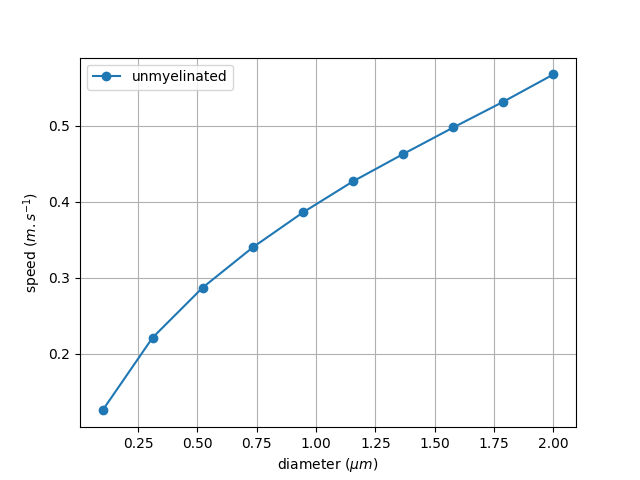
Text(42.847222222222214, 0.5, 'speed ($m.s^{-1}$)')
Let’s do the same thing but with myelinated fibers this time. Note that we need to update the fiber’s length at each new axon diameter as the node-of-ranvier distance increases with diameter.
myelinated_diameters = np.linspace(2, 20, 10)   #10 myelinated fibers with diameter ranging from 2µm to 20µm.
myelinated_speed = []

## Axon def
y = 0
z = 0
model = "MRG"

## test pulse
t_start = 1
duration = 0.1
amplitude = 5

t_sim = 5

for d in myelinated_diameters:
    L = nrv.get_length_from_nodes(d, 21)
    axon1 = nrv.myelinated(y, z, d, L, model=model)
    axon1.insert_I_Clamp(0, t_start, duration, amplitude)

    ## Simulation
    results = axon1(t_sim=t_sim)
    del axon1

    results.rasterize("V_mem")
    myelinated_speed += [results.get_avg_AP_speed()]

fig, ax  = plt.subplots()
ax.plot(myelinated_diameters, myelinated_speed, "o-", label="myelinated")
ax.legend()
ax.grid()
ax.set_xlabel(r"diameter ($\mu m$)")
ax.set_ylabel(r"speed ($m.s^{-1}$)")
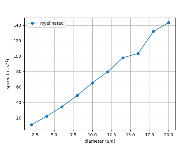
Text(38.347222222222214, 0.5, 'speed ($m.s^{-1}$)')
Myelinated and unmyelinated AP velocities can be plotted in the same figure (in log scale), clearly demonstrating the AP propagation speed gain provided by the axon’s myelin sheath.
fig, ax  = plt.subplots()
ax.loglog(unmyelinated_diameters, unmyelinated_speed, "o-", label="unmyelinated")
ax.loglog(myelinated_diameters, myelinated_speed, "o-", label="myelinated")
ax.legend()
ax.grid()
ax.set_xlabel(r"diameter ($\mu m$)")
ax.set_ylabel(r"speed ($m.s^{-1}$)")
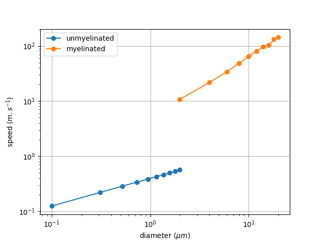
Text(31.538814019097217, 0.5, 'speed ($m.s^{-1}$)')
Effect of model on Velocity-diameter relationship
The user can choose between several unmyelinated and myelinated
computationnal models commonly found in the literature. Available
unmyelinated model are the Rattay_Aberham model (Rattay and Aberham,
1993), the HH model (Hodgkin and Huxley, 1952), the Sundt model
(Sundt et al. 2015), the Tigerholm model (Tigerholm et al. 2014),
the Schild_94 model (Schild et al. 1994) and the Schild_97 model
(Schild et al. 1997). For myelinated fibers, available myelinated models
are the MRG model (McIntyre et al., 2002), the Gaines_sensory
and Gaines_motor models (Gaines et al., 2018). Each computational
model has specific ion channels and membrane characteristics, resulting
in differences in propagation speed. Let’s see how this changes for
myelinated fibers. This typically takes between one to two minutes to
run.
myelinated_diameters = np.linspace(2, 20, 10)   #10 myelinated fibers with diameter ranging from 2µm to 20µm.

## Axon def
y = 0
z = 0

## test pulse
t_start = 1
duration = 0.1
amplitude = 5

t_sim = 5

fig, ax  = plt.subplots()

myelinated_models = ['MRG','Gaines_motor','Gaines_sensory']
for model in myelinated_models:
    myelinated_speed = []
    print(f"Simulated model: {model}")
    for d in myelinated_diameters:
        L = nrv.get_length_from_nodes(d, 21)
        axon1 = nrv.myelinated(y, z, d, L, model=model)
        axon1.insert_I_Clamp(0, t_start, duration, amplitude)
        ## Simulation
        results = axon1(t_sim=t_sim)
        del axon1
        results.rasterize("V_mem")
        myelinated_speed += [results.get_avg_AP_speed()]
    ax.plot(myelinated_diameters, myelinated_speed, "o-", label=model)

ax.legend()
ax.grid()
ax.set_xlabel(r"diameter ($\mu m$)")
ax.set_ylabel(r"speed ($m.s^{-1}$)")
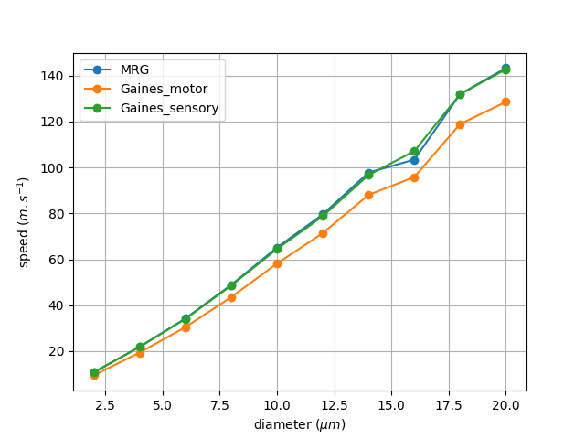
Simulated model: MRG
Simulated model: Gaines_motor
Simulated model: Gaines_sensory

Text(38.347222222222214, 0.5, 'speed ($m.s^{-1}$)')
Although not identical, the 3 models have very similar propagation speeds. Indeed, these models are very similar, Gaines’ versions being directly derived from the MRG model. Let’s do the same thing but with unmyelinated models:
unyelinated_diameters = np.linspace(0.1, 2, 10)   #10 unmyelinated fibers with diameter ranging from 0.1µm to 2µm.

## Axon def
y = 0
z = 0
L = 1000

## test pulse
t_start = 1
duration = 0.1
amplitude = 5

t_sim = 10

fig, ax  = plt.subplots()
unmyelinated_models = ["HH","Rattay_Aberham","Sundt","Tigerholm"]
for model in unmyelinated_models:
    unmyelinated_speed = []
    print(f"Simulated model: {model}")
    for d in unmyelinated_diameters:
        axon1 = nrv.unmyelinated(y, z, d, L, model=model)
        axon1.insert_I_Clamp(0, t_start, duration, amplitude)
        results = axon1(t_sim=t_sim)
        del axon1
        results.rasterize("V_mem")
        unmyelinated_speed += [results.get_avg_AP_speed()]
    ax.plot(unmyelinated_diameters, unmyelinated_speed, "o-", label=model)

ax.legend()
ax.grid()
ax.set_xlabel(r"diameter ($\mu m$)")
ax.set_ylabel(r"speed ($m.s^{-1}$)")
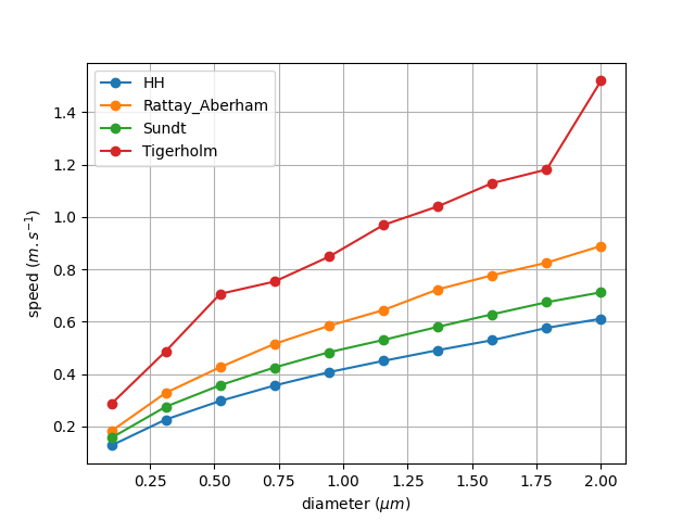
Simulated model: HH
Simulated model: Rattay_Aberham
Simulated model: Sundt
Simulated model: Tigerholm

Text(42.722222222222214, 0.5, 'speed ($m.s^{-1}$)')
On the other hand, we can see that the differences in propagation speed between the different models of unmyelinated fibers are much more pronounced. As a matter of fact, these different models were developed using different data and for different purposes, which is why they differ so much. These models are described in detail in Pelot et al. (Pelot et al. 2021).
Total running time of the script: (6 minutes 59.275 seconds)